
Natural language processing - often abbreviated NLP - is the field of machine learning focused on writing code that allows computers to understand natural human language.
NLP combines linguistics, computer programming, and machine learning helps computers read and understand human language.
In this tutorial, you will learn how to build natural language processing models in Python. You'll also learn how to perform text preprocessing in Python, and why preprocessing is such an important part of natural language processing.
Table of Contents
You can skip to a specific section of Python natural language processing tutorial using the table of contents below:
- Install The Python Natural Language Toolkit
- The Identifier and Data Set We Will Use In This Tutorial
- Examining Our Data Set
- The Libraries You Will Need In This Tutorial
-
Text Preprocessing for Natural Language Processing Models
- Removing Punctuation
- Removing Stop Words
- Performing Text Preprocessing On A Sample Message
- Building A Text Preprocessing Function
- Tokenizing Our Data Set
- Vectorizing The Data Set
- Testing Our Bag Of Words Transformation
- Building A Bag Of Words Matrix
- Normalizing the Frequency and Unit Length of the Bag Of Words Matrix
- Building our TF-IDF Matrix
- Training Our Natural Language Processing Model
- Making Predictions With Our Natural Language Processing Model
- Splitting Our Data Into Training Data and Test Data
- Building Our Data Pipeline
- Training Our Data Pipeline
- Making Predictions With Our Data Pipeline
- Measuring The Performance Of Our Data Pipeline
- The Full Code For This Tutorial
- Final Thoughts
Install The Python Natural Language Toolkit
Unlike the other Python packages we have used so far in this course, the Natural Language Toolkit does not come installed by default.
If you installed Python using the Anaconda distribution, you can install the Natural Language Toolkit with the following command in your terminal:
conda install nltkIf you installed Python using pip or another tool, you can install nltk with the following command in your terminal:
pip install nltkWith that out of the way, let's continue building our natural language processing model.
The Identifier and Data Set We Will Use In This Tutorial
This tutorial will use natural language processing to build a spam filter. To do this, we will be using the stopwords identifier that is included with the nltk library.
To start, open up a Jupyter Notebook. You'll want to first import the nltk library into your Jupyter Notebook with the following command:
import nltkNext, you will want to trigger the nltk download shell with the following statement:
nltk.download_shell()This will trigger an interactive shell environment that looks like this:
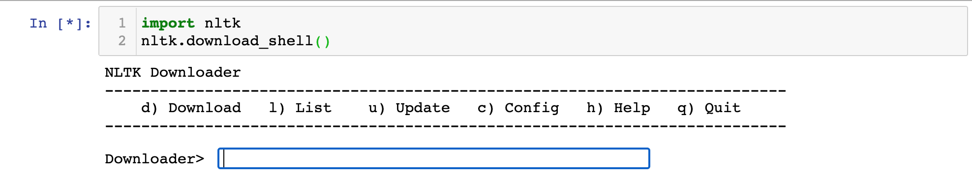
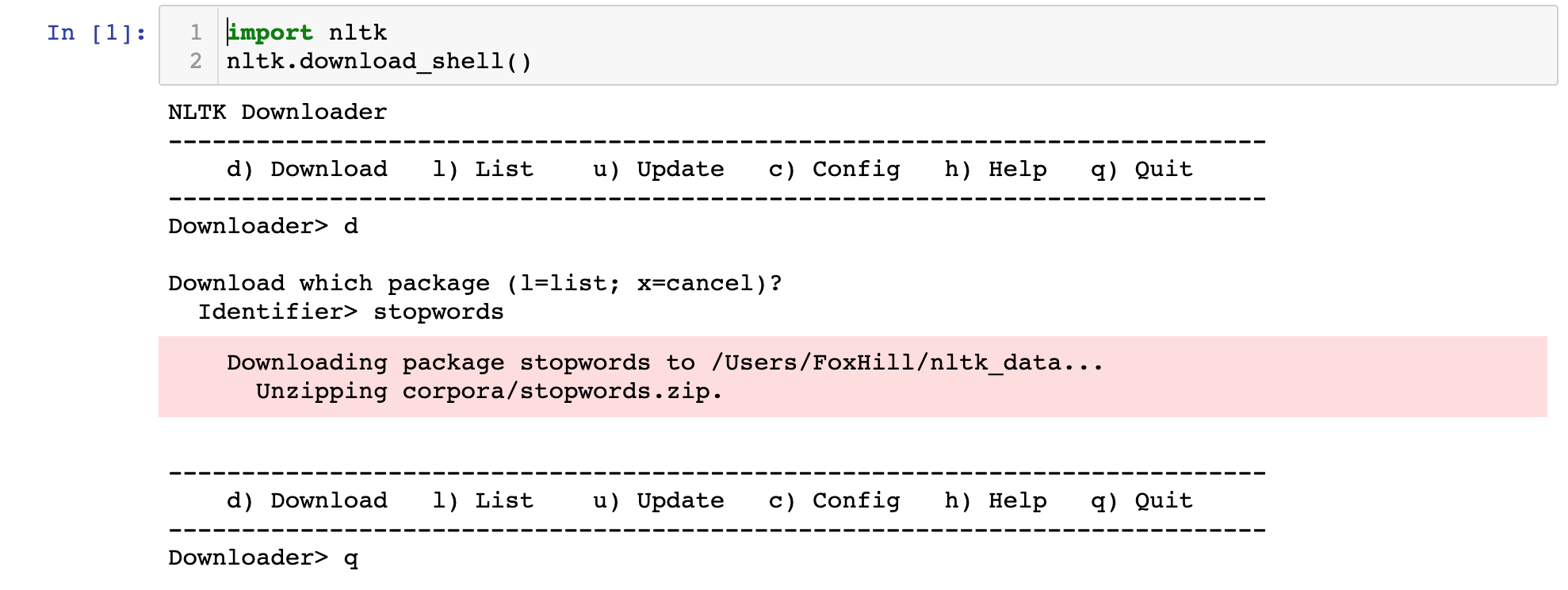
In this shell you will need to type d then Enter to specify that you're downloading a package.
From there, type in the stopwords identifier for the corpus that we are trying to download, and hit Enter again.
Pressing q and Enter once this is completed will close the interactive nltk shell.
Here is an image of what this should look like when you are done:
Our identifier has been imported. Our next step is to import our data set.
The data set we'll be using is the SMS Spam Collection Data Set made available from the UCI Machine Learning Repository. This data set is a collection of 5,574 SMS messages that have tagged as being either legitimate or spam.
The first step of importing this data set is downloading the file that contains the data. Click here to download it as a zip file. You'll want to click on the zip file after it downloads to decompress the actual file - which is called SMSSpamCollection.
Next, move this SMSSpamCollection file into the same folder as your Jupyter Notebook.
Lastly, run the following command:
data = [line.rstrip() for line in open('SMSSpamCollection')]This will create a Python list where every item in the list is a different SMS message form the SMS Spam Collection Data Set.
Examining Our Data Set
We now have a Python list named data that contains more than 5000 text messages.
Let's examining the text message with index 10 by using the data[10] command. It generates:
"ham\tI'm gonna be home soon and i don't want to talk about this stuff anymore tonight, k? I've cried enough today."This message starts with ham to indicate that it is not a spam message. In case you're not familiar, spam and ham and often used as opposites of each other.
Next the message contains \t, which implies a tab. The contents of the actual text message round out the remainder of the list item.
These tab separators indicate that our data set is stored inside of a tab-separated value file. This means that it is easy to read the data set into a pandas DataFrame!
Before that, though, we'll need to import various libraries we'll need in our script. Let's handle that next.
The Libraries You Will Need In This Tutorial
This tutorial will make use of a number of open-source Python libraries, including NumPy and pandas.
Here is a general suite of imports you should run before proceeding through the remainder of this article:
import pandas as pd

import numpy as np

import matplotlib.pyplot as plt

import seaborn as sns

%matplotlib inline
Now that we've imported our data libraries, we can now reconfigure the SMS Spam Collection Data Set into a pandas DataFrame in our Python script.
You can do this using the following statement:
data_frame = pd.read_csv('SMSSpamCollection', sep = '\t', names = ['type', 'message'])Let's now explore the data set by performing some exploratory data analysis.
Exploratory Data Analysis
Exploratory data analysis is the process of learning about a data set by calculating summary statistics and creating data visualizations.
It is an important part of any machine learning process.
Let's learn more about the SMS Spam Collection Data Set by using some basic exploratory data analysis techniques.
Counting the Unique Messages In The Data Set
Running the describe method on our pandas DataFrame will generate the following output:
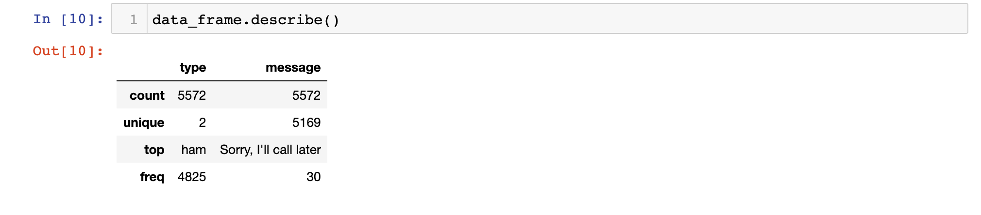
The describe method is an excellent tool for learning more about a data set.
In this case, the most interesting takeaway from using the describe method is that the number of unique messages in the data set is smaller than the number of total messages in the data set. This implies that there are duplicate messages - likely basic messages like Yes and No.
Examining The Differences Between ham and spam Messages
We can combine the pandas groupby method with the describe method to get a sense of the differences between the ham and spam categories. Here's what happens when you do this:
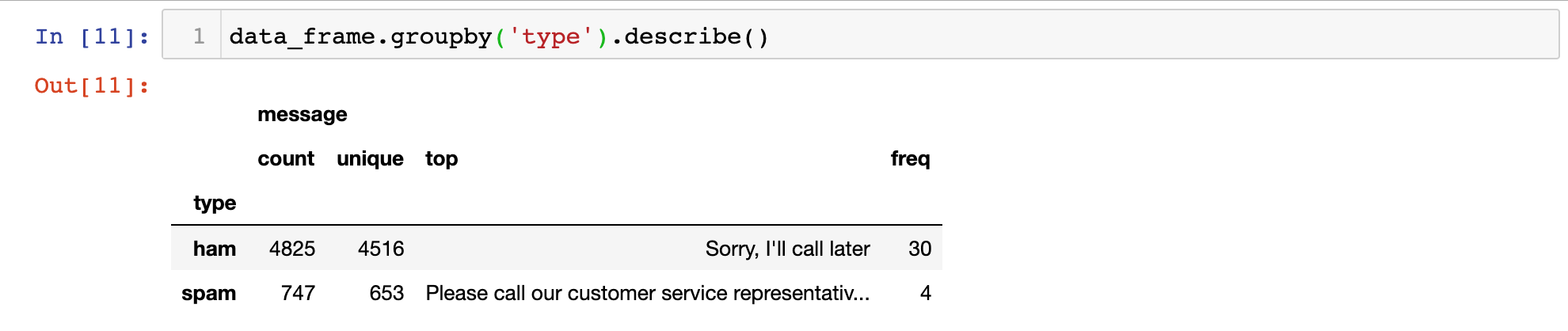
As you can see, the most common ham message is Sorry, I'll call later. The most common spam message starts with Please call our customer service representative.
We now have a basic sense of the structure of the data within our SMS Spam Collection Data Set. Let's move on to selection the features for our machine learning algorithm in the next section.
Feature Engineering & Visualizing Message Length
Feature engineering - which is the process of deciding which factors to use in training your model - is an extremely important part of building natural language processing models.
The better you understand your data set, the more likely you are to be equipped to select its best features.
To start, let's add a new column to our DataFrame that contains the length of each text message in the data set:
data_frame['message length'] = data_frame['message'].apply(len)Now that we have data on the length of each message, we can generate a plot of the distribution of message lengths using seaborn with the following statement:
sns.distplot(data_frame['message length'])This generates the following data visualization:
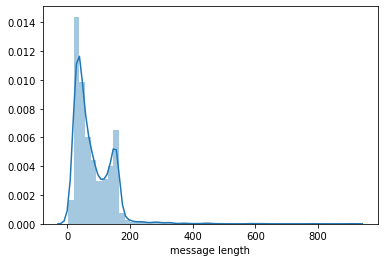
This data set seems to be bimodal in nature, which means it has two peaks when presented in a histogram. This might suggest that there are two average points - one for spam messages and one for ham messages!
Let's investigate this by creating separate subplots for both spam and ham messages:
data_frame.hist(column='message length', by='type', figsize=(13,5))This generates:
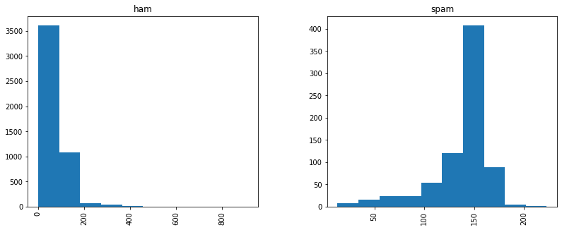
While this image is far from the most aesthetically appealing visualization we have created in this course, it does show that the two data sets have meaningfully different distributions of message length.
More specifically ,spam messages ten to be longer (they have a higher mean) and ham messages have far more dispersion.
Text Preprocessing for Natural Language Processing Models
Since the data set we are working with in this tutorial comes in the form of strings, then the classification algorithms that we have used so far in this course (like logistic regression or k-nearest neighbors) cannot be used right away.
We need to perform a process called text preprocessing to address this.
Removing Punctuation
Text preprocessing allows you to transform text into numerical formats. More specifically, we often transform documents in a corpus into a bag of words, just like we did with black dog and brown dog earlier in this course!
One of the first steps of text preprocessing is to remove punctuation - like !, ., or ? - from every document in our corpus.
To do this, we will be relying on Python's string library. Import this library into your script with the following statement:
import stringThis string library contains a Python string called string.punctuation which lists every character that is considered to be punctuation. Here's the string:
!"#$%&\'()*+,-./:;<=>?@[\\]^_`{|}~We'll use this string.punctuation object shortly to remove these punctuation characters from every document in our corpus.-
Removing Stop Words
Another important step of text preprocessing is the removal of stop words, which are non-meaningful words like the or a. The stopwords identifier that we imported from the nltk library earlier in this tutorial will be very useful for this.
We'll need to start our stop words removal process by importing the stopwords object from nltk.corpus with the following statement:
from nltk.corpus import stopwordsThis stopwords object that we've just imported is a Python class instance. It is not yet an actual list of stopwords.
We must call the words method on this object and pass in our desired language to get a list of stopwords, like this:
stopwords_list = stopwords.words('english')This new stopwords_list variable is a Python list where each element in the list is a string that is considered to be a stop word.
Performing Text Preprocessing On A Sample Message
Let's now perform our first two text preprocessing techniques - the removal of punctuation and stop words - on a sample message.
Here's the message we'll be using:
sample_message = 'This is a sample message! It has punctuation...will we be able to remove it?'First, let's remove its punctuation. We'll use Python list comprehension combined with the join method to do this.
Here's the full statement:
message_without_punctuation = ''.join([char for char in sample_message if char not in string.punctuation])This new message_without_punctuation variable now stores the following value:
'This is a sample message It has punctuation will we be able to remove it'As you can see, we have successfully removed punctuation from our sample message. Let's use a similar technique to remove stop words from the message;
cleaned_message = ' '.join([word for word in message_without_punctuation.split() if word.lower() not in stopwords_list])This cleaned_message variable now stores the following string:
'sample message punctuation able remove'This string has been cleaned of both punctuation and stop words.
Let's now formalize all of this logic into a Python function. We can then apply the function to every document in our SMS Spam Collection Data Set.
Building A Text Preprocessing Function
Let's begin by creating an empty function named preprocessor that accepts a string named message.
def preprocessor(message):Next let's write a useful docstring that explains the functionality of preprocessor:
def preprocessor(message):

    """

    This function accepts a SMS message and performs two main actions:

    1. Removes punctuation from the SMS message

    2. Removes stop words (defined by the nltk library) from the SMS message

    The function returns a Python list.

    """
Now let's add the punctuation and stop words removal functionality that we explored in the last section:
def preprocessor(message):

    """

    This function accepts a SMS message and performs two main actions:

    1. Removes punctuation from the SMS message

    2. Removes stop words (defined by the nltk library) from the SMS message

    The function returns a Python list.

    """


    message_without_punctuation = ''.join([char for char in message if char not in string.punctuation])

    return [word for word in message_without_punctuation.split(' ') if word.lower() not in stopwords.words('english')]
Now that the function has been defined, let's test the preprocessor function on our sample_message by running the following statement:
preprocessor(sample_message)This returns:
['sample', 'message', 'punctuation', 'able', 'remove']It looks like our preprocessor function is working as intended! We can now move on to applying this function to every document in our corpus.
Tokenizing Our Data Set
The action of applying a preprocessing algorithm to every document in a corpus is sometimes called tokenizing. In this section, we will tokenize the SMS messages inthe SMS Spam Collection Data Set.
To do this, we will use Python's apply method. Here's the statement to do this:
data_frame['message'] = data_frame['message'].apply(preprocessor)Note that given the size of the data set and the complexity of this function, this statement may take several seconds to complete in your Jupyter Notebook.
This tokenization step is actually included in the model we'll be using to create our bags of words later on in this tutorial, so you'll want to comment out this step and re-import your data set.
Said differently, this step was presented only to help you better understand what's happening under the hood in this natural language processing machine learning model.
Vectorizing The Data Set
The next step in our text preprocessing is to vectorize the data set, which is a fancy term that simply means transforming each message in the dataset into a bag of words.
We'll do this in three steps:
- Counting the number of times that each words appears in each method
- Normalizing the frequency so that more frequent words get lower relative weight (this is called inverse document frequency)
- Normalize the vectors to their unit length, which will allows us to compare messages with different numbers of characters in them
We will be using scikit-learn's CountVectorizer model to do this. This model converts documents within a corpus to a matrix of token counts. Note that since there are so many text messages in our data set and peoples' vocabularies are highly varied, there will be many entries of 0 in the token count matrix.
Let's begin by importing the CountVectorizer model:
from sklearn.feature_extraction.text import CountVectorizerNext, let's create an instance of the CountVectorizer class and call it bag_of_words_builder.
The CountVectorizer model takes in a number of arguments, but we can simplify our bag of words creation greatly by just passing in the argument analyzer = preprocessor, which tells the model to create the bags of words based on the preprocessor function we created earlier.
Lastly, we will call the fit method on this model and pass in the pandas Series data_frame['message'].
Here is the full statement:
bag_of_words_builder = CountVectorizer(analyzer = preprocessor).fit(data_frame['message'])Let's see how many words are in our bag of words with the following statement:
len(bag_of_words_builder.vocabulary_)This returns 11427, which is the number of unique words in our corpus.
Testing Our Bag Of Words Transformation
Let's test our bag of words transformation by applying it to the first message in the data set. To do this, first grab the first message and assign it to a variable called first_message:
first_message = data_frame['message'][0]Next, you should call the transform method on the bag_of_words_builder model and pass in first_message within an array, like this:
first_bag_of_words = bag_of_words_builder.transform([first_message])We have successfully created our first bag of words! Printing this object reveals that it looks like this:
 (0, 1111)	1

  (0, 1484)	1

  (0, 2061)	1

  (0, 4654)	1

  (0, 5218)	1

  (0, 5219)	1

  (0, 5770)	1

  (0, 6218)	1

  (0, 6907)	1

  (0, 6938)	1

  (0, 7556)	1

  (0, 7669)	1

  (0, 8338)	1

  (0, 8919)	1

  (0, 10967)	1

  (0, 11165)	1
Each entry corresponds to a word, and the number beside it shows how many times that word appears in the message. The fact that every entry in this bag of words is 1 shows that there are no duplicated words in this SMS message.
To see which words correspond to each numerical index, call the bag_of_words_builder.get_feature_names method and pass in the index you're curious about.
For example, the last word in this bag of words has index 11165. You can print the corresponding word with the following statement:
print(bag_of_words_builder.get_feature_names()[11165])This prints world, which is indeed in the SMS message. Nice!
Building A Bag Of Words Matrix
Let's now apply the transform method to every message in our data set to create a matrix that contains a bag of words for every message in the data set.
bag_of_words_matrix = bag_of_words_builder.transform(data_frame['message'])This command is fairly computationally intensive, so it may take some time to run to completion.
Normalizing the Frequency and Unit Length of the Bag Of Words Matrix
We will now normalize the frequency and unit length of each bag of words within our bag of words matrix using the TD-IDF methods described in our last section.
To do this, we will be relying on the TfidfTransformer class available from scikit-learn. Let's start by importing it:
from sklearn.feature_extraction.text import TfidfTransformerNow let's create an instance of this class and fit it to our bag of words matrix:
tfidf_builder = TfidfTransformer().fit(bag_of_words_matrix)Now let's see what happens when we use this TF-IDF model to transform the bag of words generated from the first message in our data set.
first_message_tfidf = tfidf_builder.transform(first_bag_of_words)Printing this first_message_tfidf variable generates the following output:
  (0, 11165)	0.23026685592418913

  (0, 10967)	0.19073428545061483

  (0, 8919)	0.24704652376837993

  (0, 8338)	0.17046869292195632

  (0, 7669)	0.26403384065473806

  (0, 7556)	0.31253856260694546

  (0, 6938)	0.1834692413608692

  (0, 6907)	0.15158474664662352

  (0, 6218)	0.18915557732842803

  (0, 5770)	0.24984711892976424

  (0, 5219)	0.26870593862526665

  (0, 5218)	0.29835184088197164

  (0, 4654)	0.31253856260694546

  (0, 2061)	0.24203960256420656

  (0, 1484)	0.31253856260694546

  (0, 1111)	0.2882862016308418
These numbers can be interpreted as the relative weight of each word (represented as its bag of word index) relative to all the documents in the corpus.
Building our TF-IDF Matrix
Using techniques similar to those used in the last section, we will now calculate TF-IDF values for every message in our bag of words matrix.
Here is the statement to do this:
tfidf_matrix = tfidf_builder.transform(bag_of_words_matrix)After about 2500 words of text preprocessing, we are now ready to finally start training our natural language processing model! This shows the importance of data cleaning compared to the actual machine learning techniques used in the field of natural language processing.
Training Our Natural Language Processing Model
For reasons that are outside the scope of this tutorial, it makes sense to use a multinomial naive Bayes' Theorem model to train our natural language processing model.
To start, we will want to import this model class from scikit-learn with the following command:
from sklearn.naive_bayes import MultinomialNBNow let's create an instance of this model and fit it to our tfidf_matrix variable. You will also want to pass in the labels front he original data set, which are stored in the pandas Series data_frame['type']:
spam_detector = MultinomialNB().fit(tfidf_matrix, data_frame['type'])Making Predictions With Our Natural Language Processing Model
Let's now use our natural language processing model to make predictions about whether an SMS message qualifies as spam or ham. More specifically, let's make a prediction about whether the first message in the data set is spam or ham.
We can do this by passing in the TF-IDF value for the message into a predict method called on the spam_detector object we just created, like this:
spam_detector.predict(first_message_tfidf)[0]This returns ham, which shows that the message we're examining is not spam.
You may have noticed that so far, we have not split our data set into training data and test data. The reason for this is that I wanted you to have a thorough understanding of natural language processing techniques before adding in this important step.
The rest of this tutorial will focus on how to train and test a formal natural language processing model using training data and test data.
Splitting Our Data Into Training Data and Test Data
Just like we did in our machine learning tutorial, we will now split our data set into test data and training data.
We'll use scikit-learn's train_test_split method to do this. Let's start by importing it:
from sklearn.model_selection import train_test_splitNext, we can create our training data and test data with the following statement:
x_training_data, x_test_data, y_training_data, y_test_data = train_test_split(data_frame['message'], data_frame['type'], test_size = 0.3)Now that we have divided our data, we have two choices:
- Perform the same text preprocessing techniques on each of the data splits
- Use
scikit-learn's data pipeline feature
We will be using the second choice in this tutorial.
Building Our Data Pipeline
A data pipeline allows us to perform numerous steps on a data set with very little complexity. This will make more sense as we build our data pipeline in this section.
To start, we will need to import the Pipeline class from scikit-learn:
from sklearn.pipeline import PipelineWe'll need to create an instance of this Pipeline object next. Let's give it the creative name of pipeline:
pipeline = Pipeline()This pipeline variable will hold our data pipeline, which is a list of tuples where each tuple is a transformation that should be made on the data set. Let's start by adding an empty list inside of the Pipeline class declaration:
pipeline = Pipeline([])Now we can add our first tuple.
Each tuple within a data pipeline has two elements:
- The name of the step within the data pipeline
- The operation that should be performed on each data point for that step of the pipeline
Our first step will be to use the CountVectorizer(analyzer=preprocessor) model on each element. We will call this step create_bow, since it's purpose is to create a bag of words. Here's what this tuple looks like:
('create_bow', CountVectorizer(analyzer=preprocessor))And here's what this tuple looks like when nested inside of the data pipeline:
pipeline = Pipeline([

    ('create_bow', CountVectorizer(analyzer=preprocessor))

])
Similarly, here's how we can create tuples to calculate our TD-IDF matrix and calculate our predictions using the multinational Bayes' Theorem model:
pipeline = Pipeline([

    ('create_bow', CountVectorizer(analyzer=preprocessor)),

    ('calculate_tfidf', TfidfTransformer()),

    ('make_prediction', MultinomialNB())

])
Our data pipeline is done!
This data pipeline behaves similarly to the other machine learning models we have explored in this course. We need to train it on our training data then we can use it to make predictions on our test data and verify its performance using a classification_report and a confusion_matrix.
Training Our Data Pipeline
Let's train our data pipeline. To do this, call the fit method on it and pass in our x_training_data and y_training_data variables, like this:
pipeline.fit(x_training_data, y_training_data)Making Predictions With Our Data Pipeline
Making predictions on our test data with our data pipeline is very straightforward.
Call the predict method on the pipeline object and pass in x_test_data:
predictions = pipeline.predict(x_test_data)Measuring The Performance Of Our Data Pipeline
We'll measure the performance of our data pipeline in a similar way that we measured the performance of our other classification algorithms earlier in this course: by using the classification_report and confusion_matrix functions.
Let's start by importing both of these functions:
from sklearn.metrics import classification_report

from sklearn.metrics import confusion_matrix
Now let's generate a classification_report:
classification_report(y_test_data, predictions)This generates:
             precision    recall  f1-score   support

         ham       0.95      1.00      0.98      1436

        spam       1.00      0.69      0.82       236

    accuracy                           0.96      1672

   macro avg       0.98      0.85      0.90      1672

weighted avg       0.96      0.96      0.95      1672
As you can tell from this classification_report, this model performs very well on the test data. Its precision is high for both
Now let's generate a confusion_matrix:
confusion_matrix(y_test_data, predictions)This generates:
array([[1436,    0],

       [  73,  163]])
Again, this matrix shows good performance. Of special importance is the complete lack of any false positives in the test data's predictions.
The Full Code For This Tutorial
You can view the full code for this tutorial in this GitHub repository. It is also pasted below for your reference:
#Import the stopwords identifier

import nltk

nltk.download_shell()

#Import the data set

data = [line.rstrip() for line in open('SMSSpamCollection')]

#Run our data imports

import pandas as pd

import numpy as np

import matplotlib.pyplot as plt

import seaborn as sns

%matplotlib inline

#Create our DataFrame

data_frame = pd.read_csv('SMSSpamCollection', sep = '\t', names = ['type', 'message'])

#Exploratory Data Analysis

data_frame.describe()

data_frame.groupby('type').describe()

data_frame['message length'] = data_frame['message'].apply(len)

sns.distplot(data_frame['message length'])

data_frame.hist(column='message length', by='type', figsize=(13,5))

#Text preprocessing

import string

from nltk.corpus import stopwords

stopwords_list = stopwords.words('english')

#Example of text preprocessing

sample_message = 'This is a sample message! It has punctuation... will we be able to remove it?'

message_without_punctuation = ''.join([char for char in sample_message if char not in string.punctuation])

cleaned_message = ' '.join([word for word in message_without_punctuation.split() if word.lower() not in stopwords_list])

#Building a text preprocessing function

def preprocessor(message):

    """

    This function accepts a SMS message and performs two main actions:

    1. Removes punctuation from the SMS message

    2. Removes stop words (defined by the nltk library) from the SMS message

    The function returns a Python list.

    """


    message_without_punctuation = ''.join([char for char in message if char not in string.punctuation])

    return [word for word in message_without_punctuation.split(' ') if word.lower() not in stopwords.words('english')]

#Testing the function

preprocessor(sample_message)

#Tokenizing the data set

# data_frame['message'] = data_frame['message'].apply(preprocessor)

#Vectorizing the data set

from sklearn.feature_extraction.text import CountVectorizer

bag_of_words_builder = CountVectorizer(analyzer = preprocessor).fit(data_frame['message'])

len(bag_of_words_builder.vocabulary_)

#Testing our bag of words transformation

first_message = data_frame['message'][0]

# print(first_message)

first_bag_of_words = bag_of_words_builder.transform([first_message])

# print(first_bag_of_words)

# print(bag_of_words_builder.get_feature_names()[11165])

#Creating a bag of words matrix

bag_of_words_matrix = bag_of_words_builder.transform(data_frame['message'])

#Importing the TD-IDF class

from sklearn.feature_extraction.text import TfidfTransformer

#Calculating a TF-IDF value

tfidf_builder = TfidfTransformer().fit(bag_of_words_matrix)

first_message_tfidf = tfidf_builder.transform(first_bag_of_words)

# print(first_message_tfidf)

#Building the TF-IDF matrix

tfidf_matrix = tfidf_builder.transform(bag_of_words_matrix)

#Import the multinomial naive bayes theorem class

from sklearn.naive_bayes import MultinomialNB

#Training the model

spam_detector = MultinomialNB().fit(tfidf_matrix, data_frame['type'])

#Making predictions

print("THE PREDICTION:" + spam_detector.predict(first_message_tfidf)[0])

#Splitting our data into training data and test data

from sklearn.model_selection import train_test_split

x_training_data, x_test_data, y_training_data, y_test_data = train_test_split(data_frame['message'], data_frame['type'], test_size = 0.3)

#Build our data pipeline

from sklearn.pipeline import Pipeline

pipeline = Pipeline([

    ('create_bow', CountVectorizer(analyzer=preprocessor)),

    ('calculate_tfidf', TfidfTransformer()),

    ('make_prediction', MultinomialNB())

])

#Fit the pipeline and make predictions

pipeline.fit(x_training_data, y_training_data)

predictions = pipeline.predict(x_test_data)

#Measure the performance of our natural language processing algorithm

from sklearn.metrics import classification_report

from sklearn.metrics import confusion_matrix

classification_report(y_test_data, predictions)

confusion_matrix(y_test_data, predictions)
Final Thoughts
In this tutorial, you learned how to build natural language processing models in Python.
Here is a brief summary of what you learned:
- How to install
nltkon your local machine and import it into your Python script - How to use the
download_shell()method to download thestopwordsidentifier - Learned about the importance of feature engineering and how to use exploratory data analysis to identify possible features (like
message length) in a data set - How to perform text preprocessing for a natural language processing model, including the process required to create a bag of words for each message in the SMS Spam Detection Data Set
- How to calculate TD-IDF scores
- How to build a data pipeline and make predictions with it