
The random forest is a machine learning classification algorithm that consists of numerous decision trees.
Each decision tree in the random forest contains a random sampling of features from the data set. Moreover, when building each tree, the algorithm uses a random sampling of data points to train the model.
In this tutorial, you will learn how to build your first random forest in Python. This article includes a real-world data set, a full codebase, and further instructions if you'd like to learn more about machine learning once you're finished.
Table of Contents
You can skip to a specific section of this Python random forests tutorial using the table of contents below:
- The Data Set We Will Need For This Tutorial
- The Imports We Will Need For This Tutorial
- Importing The Data Set Into Our Python Script
- Building and Training our Decision Tree Model
- Making Predictions Using Our Decision Tree Model
- Measuring the Performance of Our Decision Tree Model
- Building and Training Our Random Forests Model
- Making Predictions Using Our Random Forest Model
- Measuring the Performance of Our Decision Tree Model
- The Full Code For This Tutorial
- Final Thoughts
The Data Set We Will Need For This Tutorial
In this tutorial, we will be using a data set of kyphosis patients and building a random forest algorithm to predict whether or not patients have the disease.
You'll need to download the data set before proceeding. I have uploaded the data set to my website to make this easy for you. Simply click here to download the file. Once it's downloaded, move the file to the appropriate directory and open a Jupyter Notebook.
The Imports We Will Need For This Tutorial
We will be relying on a number of open-source software libraries to build our random forests model, including NumPy, pandas, and matplotlib. Let's start by importing those libraries with the following code:
#Numerical computing libraries

import pandas as pd

import numpy as np

#Visalization libraries

import matplotlib.pyplot as plt

import seaborn as sns

%matplotlib inline
Now that our imports have been executing, we are ready to import our data set into our Python script.
Importing The Data Set Into Our Python Script
You can import the kyphosis data set into your Python script using pandas' read_csv method, like this:
raw_data = pd.read_csv('kyphosis-data.csv')Let's take a look at the features included in this data set:
Raw_data.columnsThis returns:
Index(['Kyphosis', 'Age', 'Number', 'Start'], dtype='object')This data set represents a group of patients that previously had kyphosis, and then were tested again after having back surgery.
The Kyphosis column contains a value of present or absent depending on whether or not they had kyphosis, while the Age column contains the patient's age in months. The Number column indicates the number of vertebrae involved in the operation. The Start column describes the top-mot vertebrae that was operated on.
Now that we have imported our data set, let's move on to performing some exploratory data analysis.
Exploratory Data Analysis
Exploratory data analysis is the process of learning more about a data set before performing building machine learning models with it. It often involves calculating aggregate data or building visualizations.
Let's dig in to some brief exploratory data analysis before building and training our machine learning model.
Determining The Size Of The Data Set
One characteristic that machine learning engineers should always understand before building their models is the size of their data set.
pandas makes this very easy to determine. Simply invoke the info method on your pandas DataFrame like this:
raw_data.info()This generates:
RangeIndex: 81 entries, 0 to 80

Data columns (total 4 columns):

Kyphosis    81 non-null object

Age         81 non-null int64

Number      81 non-null int64

Start       81 non-null int64

dtypes: int64(3), object(1)

memory usage: 2.7+ KB
As you can see, there are 81 observations in this data set. This is a relatively small data set to be performing machine learning predictions on, but since this is simply an educational tutorial we are fine to proceed nonetheless.
Visualizing the Data
Since the data set is fairly small, we can use the seaborn library to easily visualize what is happening with each feature.
Here is the command to do this:
sns.pairplot(raw_data, hue = 'Kyphosis')Here is the plot that this seaborn command generates:
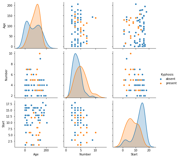
Now that we have a sense of how our data set is structured, let's divide the data set into training data and test data.
Splitting The Data Set Into Training Data and Test Data
We will be using scikit-learn's train_test_split function combined with list unpacking to create our training data and test data. Specifically, we will be using a test size of 30%.
First, let's import the train_test_split function from scikit-learn:
from sklearn.model_selection import train_test_splitNext, we need to specify the x and y data from the data set. The x data will be all of the data except for the Kyphosis column, while the y data will be the Kyphosis column by itself.
Here are the Python statements to create this division in the data set:
x = raw_data.drop('Kyphosis', axis = 1)

y = raw_data['Kyphosis']
Lastly, here is the command to create our training-test splits:
x_training_data, x_test_data, y_training_data, y_test_data = train_test_split(x, y, test_size = 0.3)We have successfully divided our data set into training data and test data.
Next up, we will continue this tutorial by building and training a decision tree algorithm on this data.
Later, we will also build a random forests model on the same training data and test data and see how its results compare with a more basic decision tree model.
Building and Training our Decision Tree Model
The first thing we need to do is import the DecisionTreeClassifier class from the tree module of scikit-learn. Run the following command to do so:
from sklearn.tree import DecisionTreeClassifierNow we need to create an instance of this class and assign it to the variable model:
model = DecisionTreeClassifier()Our model has been created. Now we need to train it using our training data.
This is done in the same way as with our linear regression, logistic regression, and K-nearest neighbors models earlier in this course: by using the fit method.
Invoke the fit method on your model object and pass in x_training_data and y_training_data, as follows:
model.fit(x_training_data, y_training_data)Our kyphosis model has been trained. Let's make some predictions using this model.
Making Predictions Using Our Decision Tree Model
To make predictions using our model object, simply call the predict method on it and pass in the x_test_data variables. You can assign these predictions to a variable named predictions.
More specifically, here is the code to do this:
predictions = model.predict(x_test_data)Now that our predictions have been made, let's assess the accuracy of our model using some of scikit-learn's built-in functionality.
Measuring the Performance of Our Decision Tree Model
We will be using scikit-learn's built-in functions classification_report and confusion_matrix to assess the performance of our decision tree machine learning model.
First, let's import these functions:
from sklearn.metrics import classification_report

from sklearn.metrics import confusion_matrix
Next, let's generate a classification_report:
print(classification_report(y_test_data, predictions))This generates:
             precision    recall  f1-score   support

      absent       0.85      0.89      0.87        19

     present       0.60      0.50      0.55         6

    accuracy                           0.80        25

   macro avg       0.72      0.70      0.71        25

weighted avg       0.79      0.80      0.79        25
We can generate a confusion_matrix in a similar manner:
print(confusion_matrix(y_test_data, predictions))This generates:
[[17  2]

 [ 3  3]]
Overall, our model seems to be doing a fairly good job of making predictions on our test data. It is only making incorrect predictions on 5 data points (2 false positives and 3 false negatives, as evidenced by the confusion_matrix).
In the next section, we will begin building a random forests model whose performance we will compare to our model object later in this tutorial.
Building and Training Our Random Forests Model
To build our random forests model, we will first need to import the model from scikit-learn. Here is the command to do this:
from sklearn.ensemble import RandomForestClassifierNext, we need to create the random forests model.
Since we do not want to overwrite the model variable that we created earlier, we will not name it model. Instead, let's name it random_forest_model:
random_forest_model = RandomForestClassifier()Note that the RandomForestClassifier class has a parameter named n_estimators that specifies the number of trees in the forest. Its default value is 100, but you can change this value if you'd like. We will be using the default value of 100 in this tutorial.
Note its time to train the random forests model. To do this, we use the fit method, as before:
random_forest_model.fit(x_training_data, y_training_data)Our random forest model has been trained. Let's move on to making some predictions with this new ensemble model.
Making Predictions Using Our Random Forest Model
Let's use the predict method to calculate some predictions using our random_forest_model object and assign them to a variable called random_forest_predictions:
random_forest_predictions = random_forest_model.predict(x_test_data)We will assess the accuracy of these predictions next.
Measuring the Performance of Our Decision Tree Model
As we did with our basic decision tree model, let's generate a classification_report and confusion_matrix.
Let's start with the classification_report:
print(classification_report(y_test_data, random_forest_predictions))Here is the output of this report:
             precision    recall  f1-score   support

      absent       0.82      0.95      0.88        19

     present       0.67      0.33      0.44         6

    accuracy                           0.80        25

   macro avg       0.74      0.64      0.66        25

weighted avg       0.78      0.80      0.77        25
Now let's generate a confusion matrix:
print(confusion_matrix(y_test_data, random_forest_predictions))Here is the output of this confusion matrix:
[[18  1]

 [ 4  2]]
In this case, our random forest has not performed significantly better than our decision tree model.
This is primarily because our data set is small. In almost all cases, random forests will perform better than basic decision trees - especially as the data set that you're using to make predictions gets larger and larger.
The Full Code For This Tutorial
You can view the full code for this tutorial in this GitHub repository. It is also pasted below for your reference:
#Numerical computing libraries

import pandas as pd

import numpy as np

#Visalization libraries

import matplotlib.pyplot as plt

import seaborn as sns

%matplotlib inline

raw_data = pd.read_csv('kyphosis-data.csv')

raw_data.columns

#Exploratory data analysis

raw_data.info()

sns.pairplot(raw_data, hue = 'Kyphosis')

#Split the data set into training data and test data

from sklearn.model_selection import train_test_split

x = raw_data.drop('Kyphosis', axis = 1)

y = raw_data['Kyphosis']

x_training_data, x_test_data, y_training_data, y_test_data = train_test_split(x, y, test_size = 0.3)

#Train the decision tree model

from sklearn.tree import DecisionTreeClassifier

model = DecisionTreeClassifier()

model.fit(x_training_data, y_training_data)

predictions = model.predict(x_test_data)

#Measure the performance of the decision tree model

from sklearn.metrics import classification_report

from sklearn.metrics import confusion_matrix

print(classification_report(y_test_data, predictions))

print(confusion_matrix(y_test_data, predictions))

#Train the random forests model

from sklearn.ensemble import RandomForestClassifier

random_forest_model = RandomForestClassifier()

random_forest_model.fit(x_training_data, y_training_data)

random_forest_predictions = random_forest_model.predict(x_test_data)

#Measure the performance of the random forest model

print(classification_report(y_test_data, random_forest_predictions))

print(confusion_matrix(y_test_data, random_forest_predictions))
Final Thoughts
In this tutorial, you learned how you build decision trees and random forests in Python.
Here is a brief summary of what you learned in this article:
- How to build a decision tree model using
scikit-learn - How to build a random forest model using
scikit-learn - That random forests typically are better predictors than decisions trees - especially with large data sets