In the last lesson of this course, you learned about the history and theory behind a linear regression machine learning algorithm.

This tutorial will teach you how to create, train, and test your first linear regression machine learning model in Python using the scikit-learn library.

Table of Contents

You can skip to a specific section of this Python machine learning tutorial using the table of contents below:

• The Data Set We Will Use in This Tutorial
• The Libraries We Will Use in This Tutorial
• Importing the Data Set
• Understanding the Data Set
• Building a Machine Learning Linear Regression Model
• Splitting our Data Set into Training Data and Test Data
• Building and Training the Model
• Making Predictions From Our Model

• Testing the Performance of our Model

  • Mean Absolute Error (MAE)
  • Mean Squared Error (MSE)
  • Root Mean Squared Error (RMSE)
• The Complete Code For This Tutorial
• Final Thoughts

The Data Set We Will Use in This Tutorial

Since linear regression is the first machine learning model that we are learning in this course, we will work with artificially-created datasets in this tutorial. This will allow you to focus on learning the machine learning concepts and avoid spending unnecessary time on cleaning or manipulating data.

More specifically, we will be working with a data set of housing data and attempting to predict housing prices. Before we build the model, we'll first need to import the required libraries.

The Libraries We Will Use in This Tutorial

The first library that we need to import is pandas, which is a portmanteau of "panel data" and is the most popular Python library for working with tabular data.

It is convention to import pandas under the alias pd. You can import pandas with the following statement:

import pandas as pd

Next, we'll need to import NumPy, which is a popular library for numerical computing. Numpy is known for its NumPy array data structure as well as its useful methods reshape, arange, and append.

It is convention to import NumPy under the alias np. You can import numpy with the following statement:

import numpy as np

Next, we need to import matplotlib, which is Python's most popular library for data visualization.

matplotlib is typically imported under the alias plt. You can import matplotlib with the following statement:

import matplotlib.pyplot as plt

%matplotlib inline

The %matplotlib inline statement will cause of of our matplotlib visualizations to embed themselves directly in our Jupyter Notebook, which makes them easier to access and interpret.

Lastly, you will want to import seaborn, which is another Python data visualization library that makes it easier to create beautiful visualizations using matplotlib.

You can import seaborn with the following statement:

import seaborn as sns

To summarize, here are all of the imports required in this tutorial:

import pandas as pd

import numpy as np

import matplotlib.pyplot as plt

%matplotlib inline

import seaborn as sns

In future lessons, I will specify which imports are necessary but I will not explain each import in detail like I did here.

Importing the Data Set

As mentioned, we will be using a data set of housing information. We will use

The data set has been uploaded to my website as a .csv file at the following URL:

https://nickmccullum.com/Housing_Data.csv

To import the data set into your Jupyter Notebook, the first thing you should do is download the file by copying and pasting this URL into your browser. Then, move the file into the same directory as your Jupyter Notebook.

Once this is done, the following Python statement will import the housing data set into your Jupyter Notebook:

raw_data = pd.read_csv('Housing_Data.csv')

This data set has a number of features, including:

• The average income in the area of the house
• The average number of total rooms in the area
• The price that the house sold for
• The address of the house

This data is randomly generated, so you will see a few nuances that might not normally make sense (such as a large number of decimal places after a number that should be an integer).

Understanding the Data Set

Now that the data set has been imported under the raw_data variable, you can use the info method to get some high-level information about the data set. Specifically, running raw_data.info() gives:

<class 'pandas.core.frame.DataFrame'>

RangeIndex: 5000 entries, 0 to 4999

Data columns (total 7 columns):

Avg. Area Income                5000 non-null float64

Avg. Area House Age             5000 non-null float64

Avg. Area Number of Rooms       5000 non-null float64

Avg. Area Number of Bedrooms    5000 non-null float64

Area Population                 5000 non-null float64

Price                           5000 non-null float64

Address                         5000 non-null object

dtypes: float64(6), object(1)

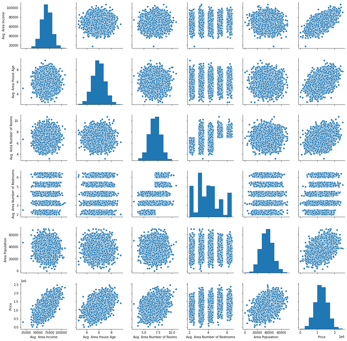
memory usage: 273.6+ KB

Another useful way that you can learn about this data set is by generating a pairplot. You can use the seaborn method pairplot for this, and pass in the entire DataFrame as a parameter. Here is the entire statement for this:

sns.pairplot(raw_data)

The output of this statement is below:

Next, let's begin building our linear regression model.

Building a Machine Learning Linear Regression Model

The first thing we need to do is split our data into an x-array (which contains the data that we will use to make predictions) and a y-array (which contains the data that we are trying to predict.

First, we should decide which columns to include. You can generate a list of the DataFrame's columns using raw_data.columns, which outputs:

Index(['Avg. Area Income', 'Avg. Area House Age', 'Avg. Area Number of Rooms',

       'Avg. Area Number of Bedrooms', 'Area Population', 'Price', 'Address'],

      dtype='object')

We will be using all of these variables in the x-array except for Price (since that's the variable we're trying to predict) and Address (since it is only contains text).

Let's create our x-array and assign it to a variable called x.

x = raw_data[['Avg. Area Income', 'Avg. Area House Age', 'Avg. Area Number of Rooms',

       'Avg. Area Number of Bedrooms', 'Area Population']]

Next, let's create our y-array and assign it to a variable called y.

y = raw_data['Price']

We have successfully divided our data set into an x-array (which are the input values of our model) and a y-array (which are the output values of our model). We'lll learn how to split our data set further into training data and test data in the next section.

Splitting our Data Set into Training Data and Test Data

scikit-learn makes it very easy to divide our data set into training data and test data. To do this, we'll need to import the function train_test_split from the model_selection module of scikit-learn.

Here is the full code to do this:

from sklearn.model_selection import train_test_split

The train_test_split data accepts three arguments:

• Our x-array
• Our y-array
• The desired size of our test data

With these parameters, the train_test_split function will split our data for us! Here's the code to do this if we want our test data to be 30% of the entire data set:

x_train, x_test, y_train, y_test = train_test_split(x, y, test_size = 0.3)

Let's unpack what is happening here.

The train_test_split function returns a Python list of length 4, where each item in the list is x_train, x_test, y_train, and y_test, respectively. We then use list unpacking to assign the proper values to the correct variable names.

Now that we have properly divided our data set, it is time to build and train our linear regression machine learning model.

Building and Training the Model

The first thing we need to do is import the LinearRegression estimator from scikit-learn. Here is the Python statement for this:

from sklearn.linear_model import LinearRegression

Next, we need to create an instance of the Linear Regression Python object. We will assign this to a variable called model. Here is the code for this:

model = LinearRegression()

We can use scikit-learn's fit method to train this model on our training data.

model.fit(x_train, y_train)

Our model has now been trained. You can examine each of the model's coefficients using the following statement:

print(model.coef_)

This prints:

[2.16176350e+01 1.65221120e+05 1.21405377e+05 1.31871878e+03

 1.52251955e+01]

Similarly, here is how you can see the intercept of the regression equation:

print(model.intercept_)

This prints:

-2641372.6673013503

A nicer way to view the coefficients is by placing them in a DataFrame. This can be done with the following statement:

pd.DataFrame(model.coef_, x.columns, columns = ['Coeff'])

The output in this case is much easier to interpret:

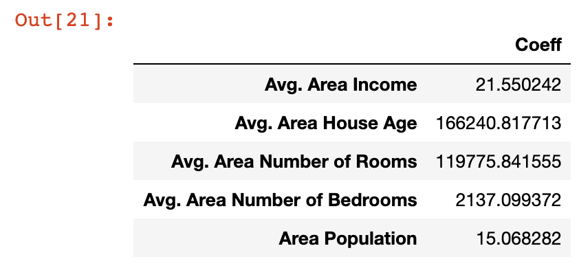
Let's take a moment to understand what these coefficients mean. Let's look at the Area Population variable specifically, which has a coefficient of approximately 15.

What this means is that if you hold all other variables constant, then a one-unit increase in Area Population will result in a 15-unit increase in the predicted variable - in this case, Price.

Said differently, large coefficients on a specific variable mean that that variable has a large impact on the value of the variable you're trying to predict. Similarly, small values have small impact.

Now that we've generated our first machine learning linear regression model, it's time to use the model to make predictions from our test data set.

Making Predictions From Our Model

scikit-learn makes it very easy to make predictions from a machine learning model. You simply need to call the predict method on the model variable that we created earlier.

Since the predict variable is designed to make predictions, it only accepts an x-array parameter. It will generate the y values for you!

Here is the code you'll need to generate predictions from our model using the predict method:

predictions = model.predict(x_test)

The predictions variable holds the predicted values of the features stored in x_test. Since we used the train_test_split method to store the real values in y_test, what we want to do next is compare the values of the predictions array with the values of y_test.

An easy way to do this is plot the two arrays using a scatterplot. It's easy to build matplotlib scatterplots using the plt.scatter method. Here's the code for this:

plt.scatter(y_test, predictions)

Here's the scatterplot that this code generates:

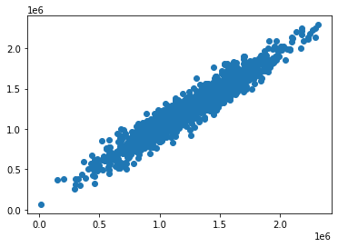
As you can see, our predicted values are very close to the actual values for the observations in the data set. A perfectly straight diagonal line in this scatterplot would indicate that our model perfectly predicted the y-array values.

Another way to visually assess the performance of our model is to plot its residuals, which are the difference between the actual y-array values and the predicted y-array values.

An easy way to do this is with the following statement:

plt.hist(y_test - predictions)

Here is the visualization that this code generates:

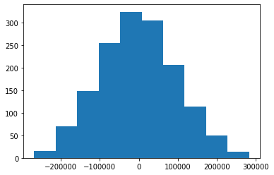
This is a histogram of the residuals from our machine learning model.

You may notice that the residuals from our machine learning model appear to be normally distributed. This is a very good sign!

It indicates that we have selected an appropriate model type (in this case, linear regression) to make predictions from our data set. We will learn more about how to make sure you're using the right model later in this course.

Testing the Performance of our Model

We learned near the beginning of this course that there are three main performance metrics used for regression machine learning models:

• Mean absolute error
• Mean squared error
• Root mean squared error

We will now see how to calculate each of these metrics for the model we've built in this tutorial. Before proceeding, run the following import statement within your Jupyter Notebook:

from sklearn import metrics

Mean Absolute Error (MAE)

You can calculate mean absolute error in Python with the following statement:

metrics.mean_absolute_error(y_test, predictions)

Mean Squared Error (MSE)

Similarly, you can calculate mean squared error in Python with the following statement:

metrics.mean_squared_error(y_test, predictions)

Root Mean Squared Error (RMSE)

Unlike mean absolute error and mean squared error, scikit-learn does not actually have a built-in method for calculating root mean squared error.

Fortunately, it really doesn't need to. Since root mean squared error is just the square root of mean squared error, you can use NumPy's sqrt method to easily calculate it:

np.sqrt(metrics.mean_squared_error(y_test, predictions))

The Complete Code For This Tutorial

Here is the entire code for this Python machine learning tutorial. You can also view it in this GitHub repository.

import pandas as pd

import numpy as np

import matplotlib.pyplot as plt

import seaborn as sns

%matplotlib inline

raw_data = pd.read_csv('Housing_Data.csv')

x = raw_data[['Avg. Area Income', 'Avg. Area House Age', 'Avg. Area Number of Rooms',

       'Avg. Area Number of Bedrooms', 'Area Population']]

y = raw_data['Price']

from sklearn.model_selection import train_test_split

x_train, x_test, y_train, y_test = train_test_split(x, y, test_size = 0.3)

from sklearn.linear_model import LinearRegression

model = LinearRegression()

model.fit(x_train, y_train)

print(model.coef_)

print(model.intercept_)

pd.DataFrame(model.coef_, x.columns, columns = ['Coeff'])

predictions = model.predict(x_test)

# plt.scatter(y_test, predictions)

plt.hist(y_test - predictions)

from sklearn import metrics

metrics.mean_absolute_error(y_test, predictions)

metrics.mean_squared_error(y_test, predictions)

np.sqrt(metrics.mean_squared_error(y_test, predictions))

Final Thoughts

In this tutorial, you learned how to create, train, and test your first linear regression machine learning algorithm.

Here is a brief summary of what you learned in this tutorial:

• How to import the libraries required to build a linear regression machine learning algorithm
• How to split a data set into training data and test data using scikit-learn
• How to use scikit-learn to train a linear regression model and make predictions using that model
• How to calculate linear regression performance metrics using scikit-learn