The K nearest neighbors algorithm is one of the world's most popular machine learning models for solving classification problems.

A common exercise for students exploring machine learning is to apply the K nearest neighbors algorithm to a data set where the categories are not known. A real-life example of this would be if you needed to make predictions using machine learning on a data set of classified government information.

In this tutorial, you will learn to write your first K nearest neighbors machine learning algorithm in Python. We will be working with an anonymous data set similar to the situation described above.

Table of Contents

You can skip to a specific section of this K nearest neighbors tutorial using the table of contents below:

• The Data Set You Will Need in This Tutorial
• The Libraries You Will Need in This Tutorial
• Importing the Data Set Into Our Python Script
• Standardizing the Data Set
• Splitting the Data Set Into Training Data and Test Data
• Training a K Nearest Neighbors Model
• Making Predictions With Our K Nearest Neighbors Algorithm
• Measuring the Accuracy of Our Model
• Choosing An Optimal K Value Using the Elbow Method
• The Full Code For This Tutorial
• Final Thoughts

The Data Set You Will Need in This Tutorial

The first thing you need to do is download the data set we will be using in this tutorial. I have uploaded the file to this website. You can access it by clicking here.

Now that you have downloaded the data set, you will want to move the file to the directory that you'll be working in. After that, open a Jupyter Notebook and we can get started writing Python code!

The Libraries You Will Need in This Tutorial

To write a K nearest neighbors algorithm, we will take advantage of many open-source Python libraries including NumPy, pandas, and scikit-learn.

Begin your Python script by writing the following import statements:

import numpy as np

import pandas as pd

import matplotlib.pyplot as plt

import seaborn as sns

%matplotlib inline

Importing the Data Set Into Our Python Script

Our next step is to import the classified_data.csv file into our Python script. The pandas library makes it easy to import data into a pandas DataFrame.

Since the data set is stored in a csv file, we will be using the read_csv method to do this:

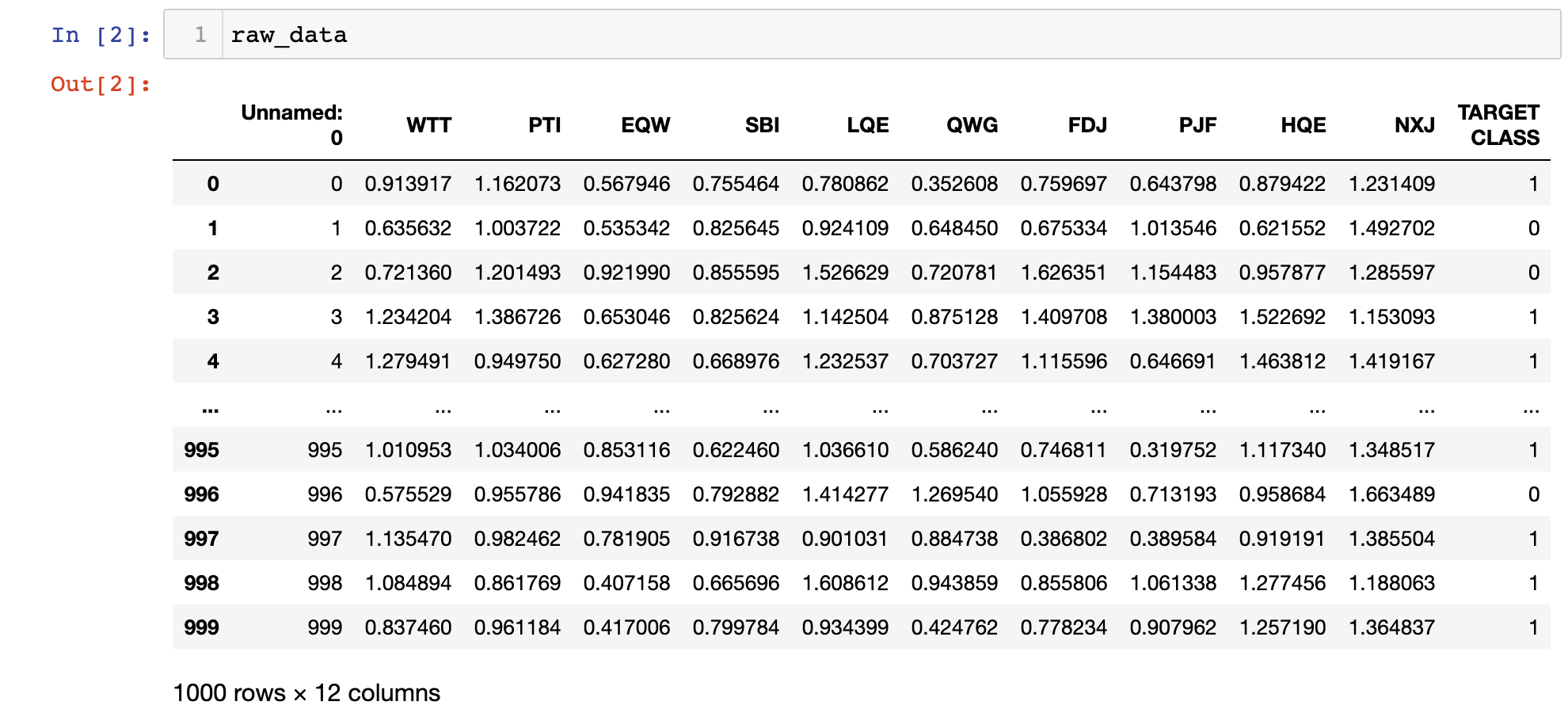
raw_data = pd.read_csv('classified_data.csv')

Printing this DataFrame inside of your Jupyter Notebook will give you a sense of what the data looks like:

You will notice that the DataFrame starts with an unnamed column whose values are equal to the DataFrame's index. We can fix this by making a slight adjustment to the command that imported our data set into the Python script:

raw_data = pd.read_csv('classified_data.csv', index_col = 0)

Next, let's take a look at the actual features that are contained in this data set. You can print a list of the data set's column names with the following statement:

print(raw_data.columns)

This returns:

Index(['WTT', 'PTI', 'EQW', 'SBI', 'LQE', 'QWG', 'FDJ', 'PJF', 'HQE', 'NXJ',

       'TARGET CLASS'],

      dtype='object')

Since this is a classified data set, we have no idea what any of these columns means. For now, it is sufficient to recognize that every column is numerical in nature and thus well-suited for modelling with machine learning techniques.

Standardizing the Data Set

Since the K nearest neighbors algorithm makes predictions about a data point by using the observations that are closest to it, the scale of the features within a data set matters a lot.

Because of this, machine learning practitioners typically standardize the data set, which means adjusting every x value so that they are roughly on the same scale.

Fortunately, scikit-learn includes some excellent functionality to do this with very little headache.

To start, we will need to import the StandardScaler class from scikit-learn. Add the following command to your Python script to do this:

from sklearn.preprocessing import StandardScaler

This function behaves a lot like the LinearRegression and LogisticRegression classes that we used earlier in this course. We will want to create an instance of this class and then fit the instance of that class on our data set.

First, let's create an instance of the StandardScaler class named scaler with the following statement:

scaler = StandardScaler()

We can now train this instance on our data set using the fit method:

scaler.fit(raw_data.drop('TARGET CLASS', axis=1))

Now we can use the transform method to standardize all of the features in the data set so they are roughly the same scale. We'll assign these scaled features to the variable named scaled_features:

scaled_features = scaler.transform(raw_data.drop('TARGET CLASS', axis=1))

This actually creates a NumPy array of all the features in the data set, and we want it to be a pandas DataFrame instead.

Fortunately, this is an easy fix. We'll simply wrap the scaled_features variable in a pd.DataFrame method and assign this DataFrame to a new variable called scaled_data with an appropriate argument to specify the column names:

scaled_data = pd.DataFrame(scaled_features, columns = raw_data.drop('TARGET CLASS', axis=1).columns)

Now that we have imported our data set and standardized its features, we are ready to split the data set into training data and test data.

Splitting the Data Set Into Training Data and Test Data

We will use the train_test_split function from scikit-learn combined with list unpacking to create training data and test data from our classified data set.

First, you'll need to import train_test_split from the model_validation module of scikit-learn with the following statement:

from sklearn.model_selection import train_test_split

Next, we will need to specify the x and y values that will be passed into this train_test_split function.

The x values will be the scaled_data DataFrame that we created previously. The y values will be the TARGET CLASS column of our original raw_data DataFrame.

You can create these variables with the following statements:

x = scaled_data

y = raw_data['TARGET CLASS']

Next, you'll need to run the train_test_split function using these two arguments and a reasonable test_size. We will use a test_size of 30%, which gives the following parameters for the function:

x_training_data, x_test_data, y_training_data, y_test_data = train_test_split(x, y, test_size = 0.3)

Now that our data set has been split into training data and test data, we're ready to start training our model!

Training a K Nearest Neighbors Model

Let's start by importing the KNeighborsClassifier from scikit-learn:

from sklearn.neighbors import KNeighborsClassifier

Next, let's create an instance of the KNeighborsClassifier class and assign it to a variable named model

This class requires a parameter named n_neighbors, which is equal to the K value of the K nearest neighbors algorithm that you're building. To start, let's specify n_neighbors = 1:

model = KNeighborsClassifier(n_neighbors = 1)

Now we can train our K nearest neighbors model using the fit method and our x_training_data and y_training_data variables:

model.fit(x_training_data, y_training_data)

Now let's make some predictions with our newly-trained K nearest neighbors algorithm!

Making Predictions With Our K Nearest Neighbors Algorithm

We can make predictions with our K nearest neighbors algorithm in the same way that we did with our linear regression and logistic regression models earlier in this course: by using the predict method and passing in our x_test_data variable.

More specifically, here's how you can make predictions and assign them to a variable called predictions:

predictions = model.predict(x_test_data)

Let's explore how accurate our predictions are in the next section of this tutorial.

Measuring the Accuracy of Our Model

We saw in our logistic regression tutorial that scikit-learn comes with built-in functions that make it easy to measure the performance of machine learning classification models.

Let's import two of these functions (classification_report and confuson_matrix) into our report now:

from sklearn.metrics import classification_report

from sklearn.metrics import confusion_matrix

Let's work through each of these one-by-one, starting with the classfication_report. You can generate the report with the following statement:

print(classification_report(y_test_data, predictions))

This generates:

             precision    recall  f1-score   support

           0       0.94      0.85      0.89       150

           1       0.86      0.95      0.90       150

    accuracy                           0.90       300

   macro avg       0.90      0.90      0.90       300

weighted avg       0.90      0.90      0.90       300

Similarly, you can generate a confusion matrix with the following statement:

print(confusion_matrix(y_test_data, predictions))

This generates:

[[141  12]

 [ 18 129]]

Looking at these performance metrics, it looks like our model is already fairly performant. It can still be improved.

In the next section, we will see how we can improve the performance of our K nearest neighbors model by choosing a better value for K.

Choosing An Optimal K Value Using the Elbow Method

In this section, we will use the elbow method to choose an optimal value of K for our K nearest neighbors algorithm.

The elbow method involves iterating through different K values and selecting the value with the lowest error rate when applied to our test data.

To start, let's create an empty list called error_rates. We will loop through different K values and append their error rates to this list.

error_rates = []

Next, we need to make a Python loop that iterates through the different values of K we'd like to test and executes the following functionality with each iteration:

• Creates a new instance of the KNeighborsClassifier class from scikit-learn
• Trains the new model using our training data
• Makes predictions on our test data
• Calculates the mean difference for every incorrect prediction (the lower this is, the more accurate our model is)

Here is the code to do this for K values between 1 and 100:

for i in np.arange(1, 101):

    new_model = KNeighborsClassifier(n_neighbors = i)

    new_model.fit(x_training_data, y_training_data)

    new_predictions = new_model.predict(x_test_data)

    error_rates.append(np.mean(new_predictions != y_test_data))

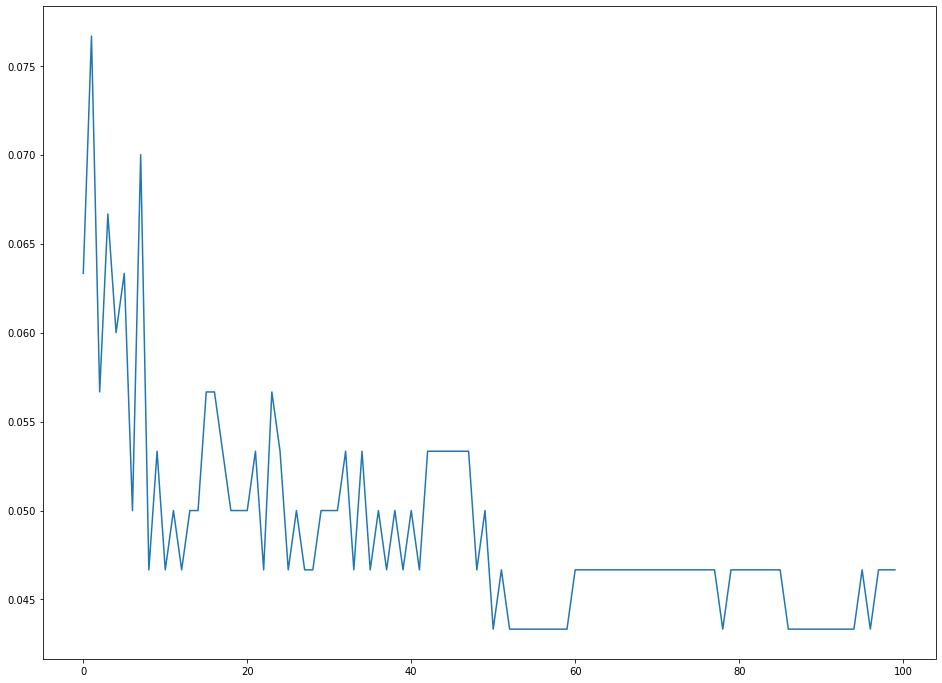
Let's visualize how our error rate changes with different K values using a quick matplotlib visualization:

plt.plot(error_rates)

As you can see, our error rates tend to be minimized with a K value of approximately 50. This means that 50 is a suitable choice for K that balances both simplicity and predictive power.

The Full Code For This Tutorial

You can view the full code for this tutorial in this GitHub repository. It is also pasted below for your reference:

#Common imports

import numpy as np

import pandas as pd

import matplotlib.pyplot as plt

import seaborn as sns

%matplotlib inline

#Import the data set

raw_data = pd.read_csv('classified_data.csv', index_col = 0)

#Import standardization functions from scikit-learn

from sklearn.preprocessing import StandardScaler

#Standardize the data set

scaler = StandardScaler()

scaler.fit(raw_data.drop('TARGET CLASS', axis=1))

scaled_features = scaler.transform(raw_data.drop('TARGET CLASS', axis=1))

scaled_data = pd.DataFrame(scaled_features, columns = raw_data.drop('TARGET CLASS', axis=1).columns)

#Split the data set into training data and test data

from sklearn.model_selection import train_test_split

x = scaled_data

y = raw_data['TARGET CLASS']

x_training_data, x_test_data, y_training_data, y_test_data = train_test_split(x, y, test_size = 0.3)

#Train the model and make predictions

from sklearn.neighbors import KNeighborsClassifier

model = KNeighborsClassifier(n_neighbors = 1)

model.fit(x_training_data, y_training_data)

predictions = model.predict(x_test_data)

#Performance measurement

from sklearn.metrics import classification_report

from sklearn.metrics import confusion_matrix

print(classification_report(y_test_data, predictions))

print(confusion_matrix(y_test_data, predictions))

#Selecting an optimal K value

error_rates = []

for i in np.arange(1, 101):

    new_model = KNeighborsClassifier(n_neighbors = i)

    new_model.fit(x_training_data, y_training_data)

    new_predictions = new_model.predict(x_test_data)

    error_rates.append(np.mean(new_predictions != y_test_data))

plt.figure(figsize=(16,12))

plt.plot(error_rates)

Final Thoughts

In this tutorial, you learned how to build your first K nearest neighbors machine learning model in Python.

Here is a brief summary of what you learned in this tutorial:

• How classified data is a common tool used to teach students how to solve their first K nearest neighbor problems
• Why it's important to standardize your data set when building K nearest neighbor models
• How to split your data set into training data and test data using the train_test_split function
• How to train your first K nearest neighbors model and make predictions with it
• How to measure the performance of a K nearest neighbors model
• How to use the elbow method to select an optimal value of K in a K nearest neighbors model