Long short-term memory networks (LSTMs) are a type of recurrent neural network used to solve the vanishing gradient problem.

They differ from "regular" recurrent neural networks in important ways.

This tutorial will introduce you to LSTMs. Later in this course, we will build and train an LSTM from scratch.

Table of Contents

You can skip to a specific section of this LSTM tutorial using the table of contents below:

• The History of LSTMs
• How LSTMs Solve The Vanishing Gradient Problem
• How LSTMs Work

• Variations of LSTM Architectures

  • The Peephole Variation
  • The Coupled Gate Variation
• Other LSTM Variations
• Final Thoughts

The History of LSTMs

As we alluded to in the last section, the two most important figures in the field of LSTMs are Sepp Hochreiter and Jürgen Schmidhuber.

The latter was the former's PhD supervisor at the Technical University of Munich in Germany.

Hochreiter's PhD thesis introduced LSTMs to the world for the first time.

How LSTMs Solve The Vanishing Gradient Problem

In the last tutorial, we learned how the Wrec term in the backpropagation algorithm can lead to either a vanishing gradient problem or an exploding gradient problem.

We explored various possible solutions for this problem, including penalties, gradient clipping, and even echo state networks. LSTMs are the best solution.

So how do LSTMs work? They simply change the value of Wrec.

In our explanation of the vanishing gradient problem, you learned that:

• When Wrec is small, you experience a vanishing gradient problem
• When Wrec is large, you experience an exploding gradient problem

We can actually be much more specific:

• When Wrec < 1, you experience a vanishing gradient problem
• When Wrec > 1, you experience an exploding gradient problem

This makes sense if you think about the multiplicative nature of the backpropagation algorithm.

If you have a number that is smaller than 1 and you multiply it against itself over and over again, you'll end up with a number that vanishes. Similarly, multiplying a number greater than 1 against itself many times results in a very large number.

To solve this problem, LSTMs set Wrec = 1. There is certainly more to LSTMS than setting Wrec = 1, but this is definitely the most important change that this specification of recurrent neural networks makes.

How LSTMs Work

This section will explain how LSTMs work. Before proceeding ,it's worth mentioning that I will be using images from Christopher Olah's blog post Understanding LSTMs, which was published in August 2015 and has some of the best LSTM visualizations that I have ever seen.

To start, let's consider the basic version of a recurrent neural network:

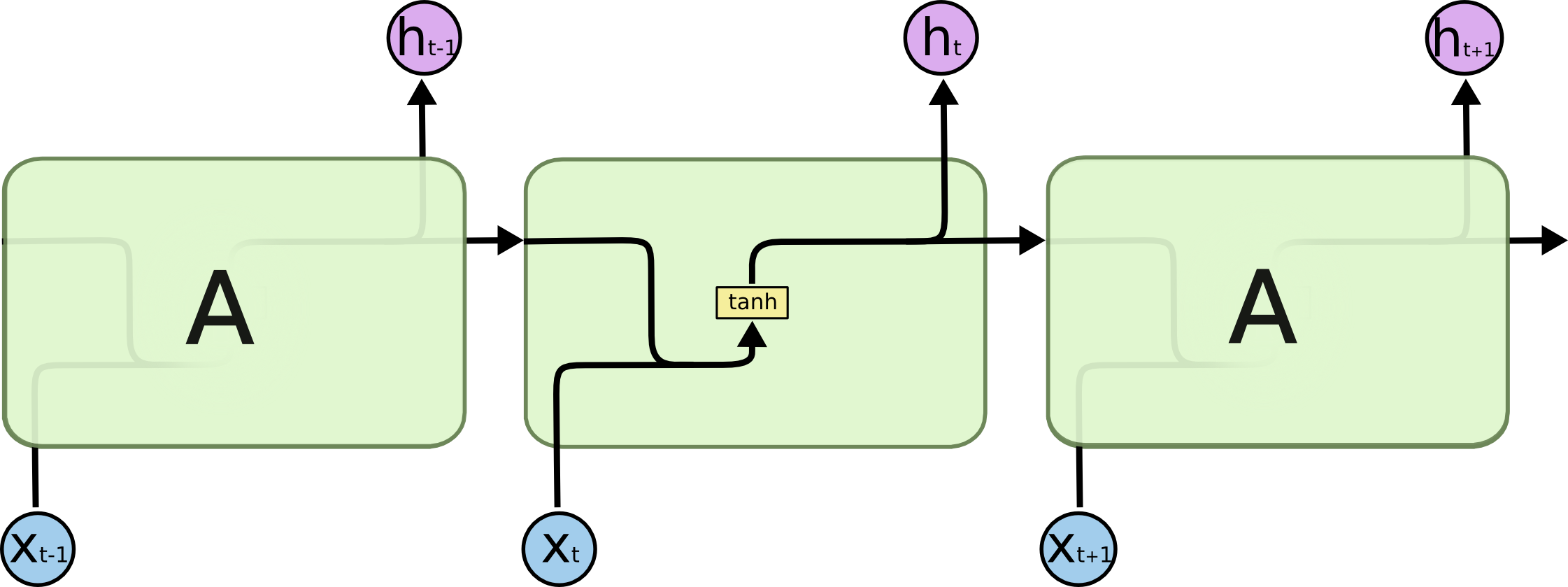
This neural network has neurons and synapses that transmit the weighted sums of the outputs from one layer as the inputs of the next layer. A backpropagation algorithm will move backwards through this algorithm and update the weights of each neuron in response to he cost function computed at each epoch of its training stage.

By contrast, here is what an LSTM looks like:

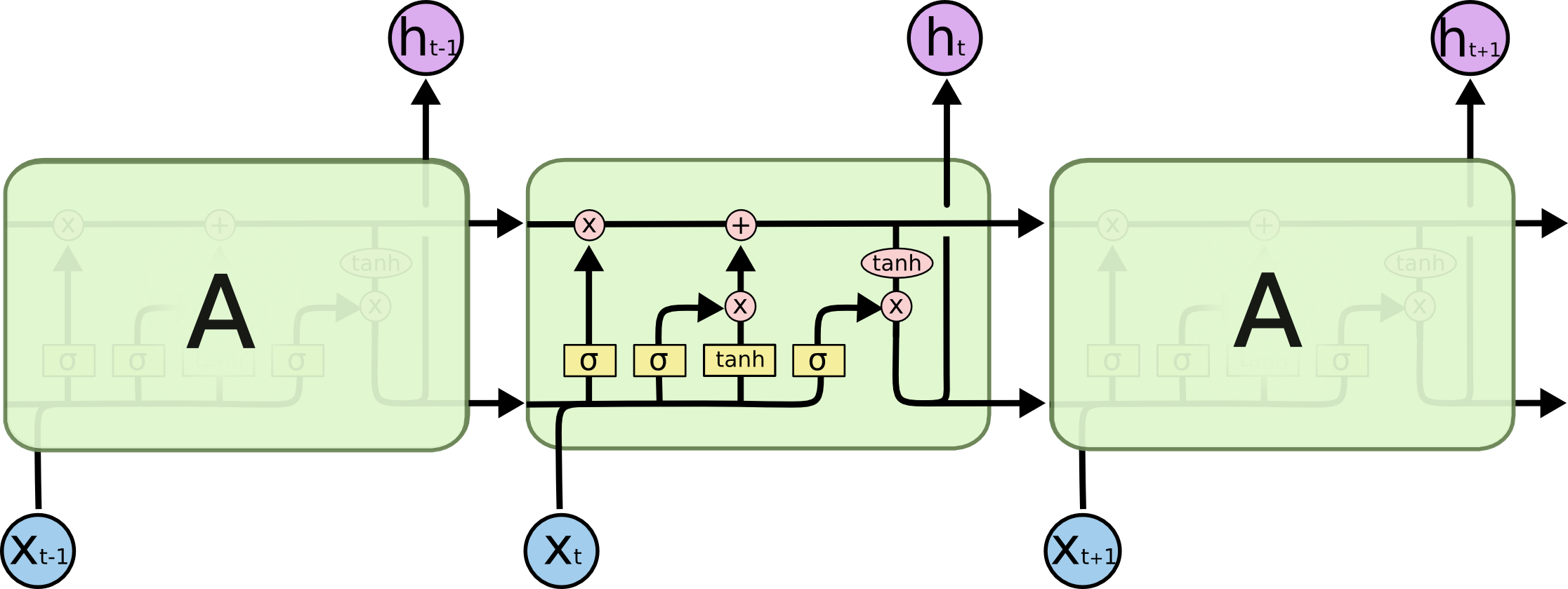
As you can see, an LSTM has far more embedded complexity than a regular recurrent neural network. My goal is to allow you to fully understand this image by the time you've finished this tutorial.

First, let's get comfortable with the notation used in the image above:

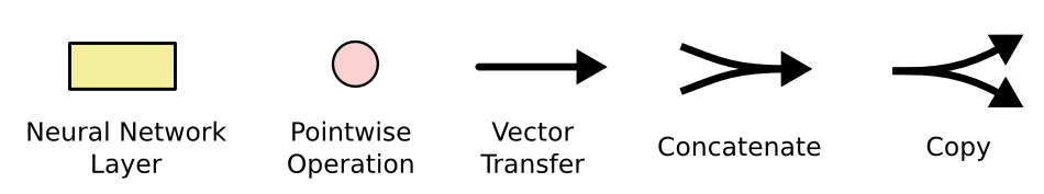
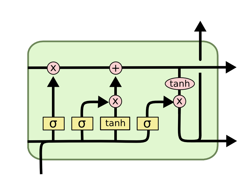
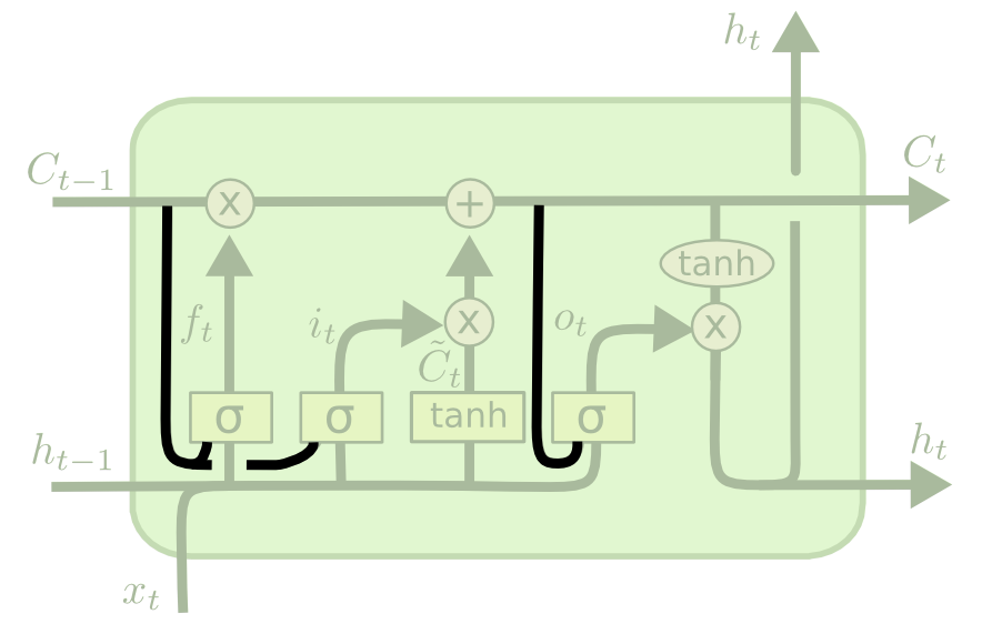
Now that you have a sense of the notation we'll be using in this LSTM tutorial, we can start examining the functionality of a layer within an LSTM neural net. Each layer has the following appearance.

Before we dig into the functionality of nodes within an LSTM neural network, it's worth noting that every input and output of these deep learning models is a vector. In Python, this is generally represented by a NumPy array or another one-dimensional data structure.

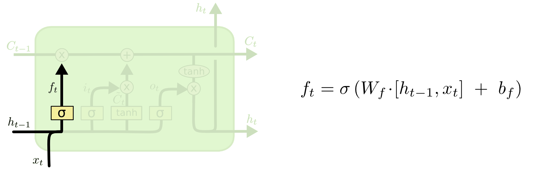
The first thing that happens within an LSTM is the activation function of the forget gate layer. It looks at the inputs of the layer (labelled xt for the observation and ht for the output of the previous layer of the neural network) and outputs either 1 or 0 for every number in the cell state from the previous layer (labelled Ct-1).

Here's a visualization of the activation of the forget gate layer:

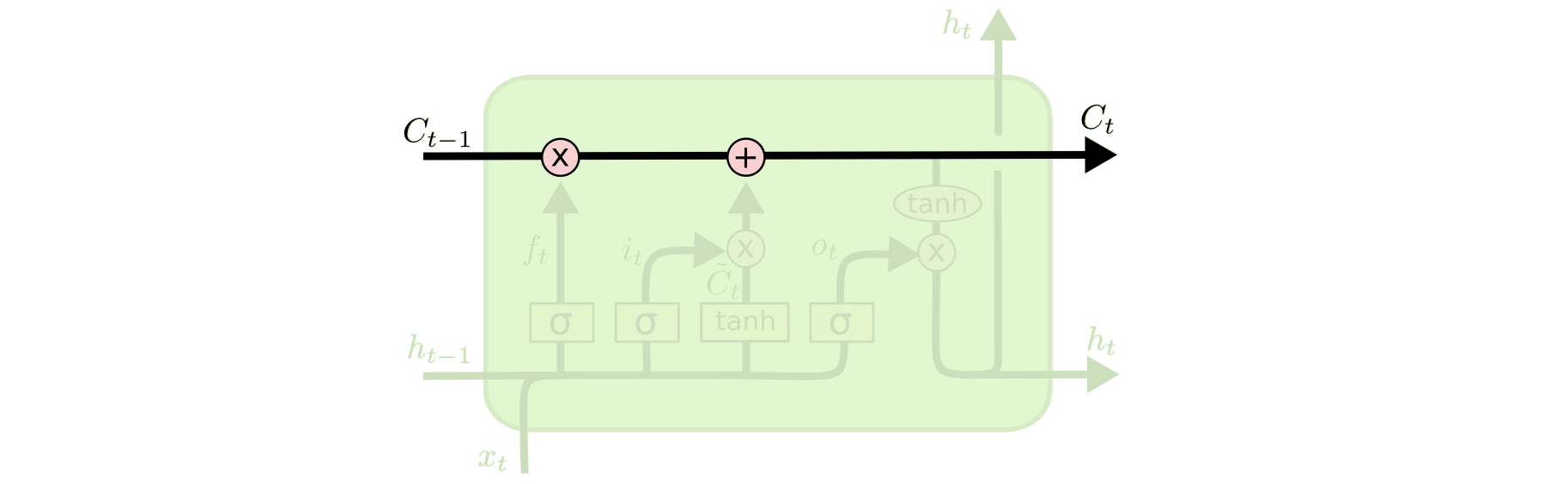
We have not discussed cell state yet, so let's do that now. Cell state is represented in our diagram by the long horizontal line that runs through the top of the diagram. As an example, here is the cell state in our visualizations:

The cell state's purpose is to decide what information to carry forward from the different observations that a recurrent neural network is trained on. The decision of whether or not to carry information forward is made by gates - of which the forget gate is a prime example. Each gate within an LSTM will have the following appearance:

The σ character within these gates refers to the Sigmoid function, which you have probably seen used in logistic regression machine learning models. The sigmoid function is used as a type of activation function in LSTMs that determines what information is passed through a gate to affect the network's cell state.

By definition, the Sigmoid function can only output numbers between 0 and 1. It's often used to calculate probabilities because of this. In the case of LSTM models, it specifies what proportion of each output should be allowed to influence the sell state.

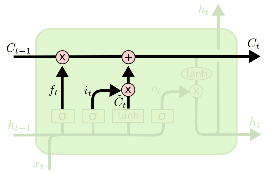
The next two steps of an LSTM model are closely related: the input gate layer and the tanh layer. These layers work together to determine how to update the cell state. At the same time, the last step is completed, which allows the cell to determine what to forget about the last observation in the data set.

Here is a visualization of this process:

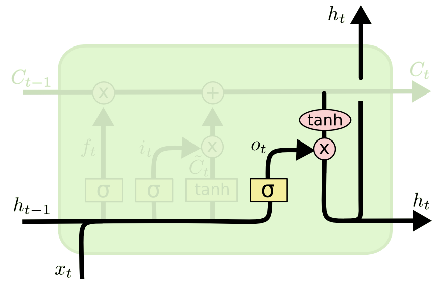
The last step of an LSTM determines the output for this observation (denoted ht). This step runs through both a sigmoid function and a hyperbolic tangent function. It can be visualized as follows:

That concludes the process of training a single layer of an LSTM model. As you might imagine, there is plenty of mathematics under the surface that we have glossed over. The point of this article is to broadly explain how LSTMs work, not for you to deeply understand each operation in the process.

Variations of LSTM Architectures

I wanted to conclude this tutorial by discussing a few different variations of LSTM architecture that are slightly different from the basic LSTM that we've discussed so far.

As a quick recap, here is what a generalized node of an LSTM looks like:

The Peephole Variation

Perhaps the most important variation of the LSTM architecture is the peephole variant, which allows the gate layers to read data from the cell state.

Here is a visualization of what the peephole varant might look like.

Note that while this diagram adds a peephole to every gate in the recurrent neural network, you could also add peepholes to some gates and not other gates.

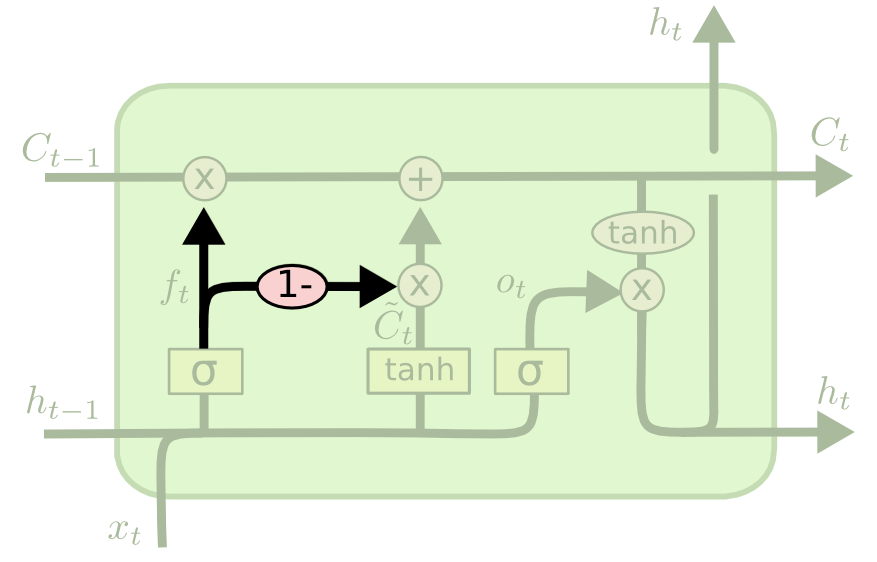
The Coupled Gate Variation

There is another variation of the LSTM architecture where the model makes the decision of what to forget and what to add new information to together. In the original LSTM model, these decisions were made separately.

Here is a visualization of what this architecture looks like:

Other LSTM Variations

These are only two examples of variants to the LSTM architecture. There are many more. A few are listed below:

• Gated Recurrent Units (GRUs)
• Depth Gated RNNs
• Clockwork RNNs

Final Thoughts

In this tutorial, you had your first exposure to long short-term memory networks (LSTMs).

Here is a brief summary of what you learned:

• A (very) brief history of LSTMs and the role that Sepp Hochreiter and Jürgen Schmidhuber played in their development
• How LSTMs solve the vanishing gradient problem
• How LSTMs work
• The role of gates, sigmoid functions, and the hyperbolic tangent function in LSTMs
• A few of the most popular variations of the LSTM architecture