
So far in this course, you have learned about the fundamentals of convolutional neural networks, including:
- The role of a convolution function in convolutional neural networks
- How
input imagesare transformed intofeature mapsusing afeature detectormatrix - How the flattening and full connection steps are used to pipe the image data into an artificial neural network that makes the final prediction
All of this was highly theoretical. I would not blame you if you found this boring or impractical.
Fortunately, it's now time to build our first convolutional neural network! More specifically, this tutorial will teach you how to build and train your first convolutional neural network to recognize cats and dogs from an image database.
Table of Contents
You can skip to a specific section of this Python convolutional neural network tutorial using the table of contents below:
- The Data Set You Will Need For This Tutorial
- The Libraries You Will Need For This Tutorial
-
Building Our Convolutional Neural Network
- Adding Our Convolutional Layer
- Adding Our Max Pooling Layer
- Adding Another Convolutional Layer and Pooling Layer
- Adding The Flattening Layer To Our Convolutional Neural Network
- Adding The Full Connection Layer To Our Convolutional Neural Network
- Adding The Output Layer To Our Convolutional Neural Network
- Training the Convolutional Neural Network
- Making Predictions With Our Convolutional Neural Network
- The Full Code For This Tutorial
- Final Thoughts
The Data Set You Will Need For This Tutorial
This tutorial will teach you how to build a convolutional neural network to make predictions about whether an image contains a cat or a dog.
To do this, you will need a data set to train the model. I have stored the data set for this tutorial in a GitHub repository. You can click here to access the repository.
Here's what the repository contains:
- A folder called
training_datathat holds 4000 images of cats and 4000 images of dogs - A folder called
test_datathat contains 1000 images of cats and 1000 images of dogs - A folder called
predictionsthat 1 image of a cat and 1 image of a dog. We will use the images in thispredictionsfolder to make single predictions using our trained model later in this tutorial.
Every image in this data set is a .jpg file.
I would recommend cloning the repository to your local machine and opening a Jupyter Notebook in the same folder. Once your Notebook is open, you can move on to importing the various libraries we'll use in this tutorial.
The Libraries You Will Need For This Tutorial
This convolutional neural network tutorial will make use of a number of open-source Python libraries, including NumPy and (most importantly) TensorFlow.
The only import that we will execute that may be unfamiliar to you is the ImageDataGenerator function that lives inside of the keras.preprocessing.image module. According to its documentation, the purpose of this function is to "Generate batches of tensor image data with real-time data augmentation." You will see the import of this function included in the code cell below.
Let's now import these libraries into our Python script.
import numpy as np

import tensorflow as tf

from tensorflow.keras.preprocessing.image import ImageDataGenerator
Now that our libraries have been imported, we can move on to preprocessing the data wel'l use in our convolutional neural network.
Preprocessing Our Data
The process that we will use to preprocess our training data will be slightly different than the process we'll use on our test data.
The reason for this is that to avoid overfitting, we will add an extra transformation to the training data images.
Overfitting is a common problem in machine learning and deep learning and is characterized by having very high accuracy on the training data and much lower accuracy on the test data.
With that disclaimer out of the way, let's start by preprocessing our training data!
Preprocessing the Training Data
The transformations that we will apply to our training data with the goal of avoiding overfitting are more simple than you might imagine. They are simple image transformations like:
- Rotations
- Cropping
- Zooming
These transformations are known as geographical transformations or geographic transformations. The broader process of modifying the original data set to avoid overfitting is called image augmentation.
The tool that we will use for image preprocessing is called the ImageDataGenerator class, which we imported earlier in this tutorial.
This function is capable of applying a number of different transformations. For simplicity's sake, we will use three. The transformations and their definitions (from the keras documentation) are shown below:
zoom_range: Float or [lower, upper]. Range for random zoom. If a float, [lower, upper] = [1-zoomrange, 1+zoomrange].horizontal_flip: Boolean. Randomly flip inputs horizontally.shear_range: Float. Shear Intensity (Shear angle in counter-clockwise direction in degrees)
The only other argument that the ImageDataGenerator class needs is rescale = 1/255, which scales every pixel in the image such that its value lies between 0 and 255 - which, as you'll recall from earlier in this course, is required for convolutional neural networks.
With all of this out of the way, let's create an instance of the ImageDataGenerator class called training_generator with a 20% shear range, a 20% zoom range, and a horizontal flip:
training_generator = ImageDataGenerator(

                        rescale = 1/255,

                        shear_range = 0.2,

                        zoom_range = 0.2,

                        horizontal_flip = True)
We've now created an object that can be used to perform image augmentation on our data set. However, the augmentation has not yet been done. We do not yet have the training data we'll use to train our convolutional neural network.
To generate our data, we'll need to call the flow_from_directory method on our new training_generator object. This method takes a number of parameters which I have specified below. This method will apply the necessary image augmentation techniques to our training data.
training_set = training_generator.flow_from_directory('training_data',

                                                 target_size = (64, 64),

                                                 batch_size = 32,

                                                 class_mode = 'binary')
Let's examine each of the parameters from this method one-by-one:
- The first parameter is the folder that the training data is contained in
- The
target_sizevariable contains the dimensions that each image in the data set will be resized to - The
batch_sizevariable represents the size of batches of data that the method will be applied to - The
class_modespecifies which time of classifier you're building. The two main options arebinary(for two classes) orcategorical(for two or more classes). There are other options which you can read about in the keras documentation if desired.
Once you run this command, your Jupyter Notebook should print the following output:
Found 8000 images belonging to 2 classes.Now that this is done, we can move on to preprocessing our test data.
Preprocessing the Test Data
As mentioned, we will not be applying image augmentation techniques to our test data. We want the test data to remain unchanged (which would be the case if our machine learning model was deployed in production).
Preprocessing our test data is comprised of two steps:
- Creating a new
ImageDataGeneratorclass that excludes the image augmentation arguments that we used on our training data - Applying the same
flow_from_directorymethod to theImageDataGeneratorclass that was just created
Here is the code to do this:
#Preprocessing the test set

test_generator = ImageDataGenerator(rescale = 1./255)

test_set = test_generator.flow_from_directory('test_data',

                                            target_size = (64, 64),

                                            batch_size = 32,

                                            class_mode = 'binary')
In this case, the following output will be printed in your Jupyter Notebook:
Found 2000 images belonging to 2 classes.Our data preprocessing is complete. We can now move on to building and training our convolutional neural network!
Building Our Convolutional Neural Network
Building our convolutional neural network will follow a similar strategy as when we built our artificial neural network earlier in this course.
We will start by initializing an instance of the Sequential class from keras. This class lives within the models module of keras, and keras lives within the TensorFlow library that we imported under the alias tf.
Putting all this together, the CNN initialization command becomes:
cnn = tf.keras.models.Sequential()We will now add various layers to this convolutional neural network object before training the neural network in a later step.
Adding Our Convolutional Layer
You will probably recall that we can add layers to a neural network using the add method. Let's start by creating a blank add method using our cnn object:
cnn.add()What parameter needs to be passed in to this add method?
As you might image, we need to specify the characteristics of our convolutional layer for the first layer of this neural network. TensorFlow contains a built-in object designed specifically for building convolutional layer.
This object lives within the layers module of keras. It is called Conv2D. Here is how you would initialize this object within the add method we just created:
cnn.add(tf.keras.layers.Conv2D())This Conv2D object needs to accept various parameters. They are:
filters: the number of feature detectors you want to use in your convolutional neural network. We will use 32 different feature detectors in this tutorial, which is a classic choice for image recognition.kernal: the size of each feature detector. Since feature detectors are square matrices, thiskernalparameter represents the length of both the matrix's columns and the matrix's rows. We will be using a parameter of3, which means that each of our feature detectors will be a3x3matrix.activation: this represents the activation function that will be used by our convolutional neural network. We will use a parameter ofrelu.input_shape: this represents the dimensions of the inputs to our convolutional neural network. Since we're working with colored images of dimension64x64, ourinput_shapewill be[64, 64, 3]. The3represents the three different colors (red, green, and blue) represented in each image. If we were working with black-and-white images, ourinput_shapeparameter would be[64, 64, 1].
Putting all of this together, we can add the convolutional layer to our convolutional neural network with the following command:
cnn.add(tf.keras.layers.Conv2D(filters=32, kernel_size=3, activation='relu', input_shape=[64, 64, 3]))Our convolutional layer has now been added to our convolutional neural network. Let's move on to our next layer, which will apply max pooling to our data set.
Adding Our Max Pooling Layer
As before, let's start by adding an empty add method to our convolutional neural network:
cnn.add()The parameter that we will pass in to this add method will be another object that lives inside the layers module of the keras library. This time, the class name is MaxPool2D.
Here's how you can instantiate the class inside the add method without specifying any parameters:
cnn.add(tf.keras.layers.MaxPool2D())The MaxPool2D module accepts many parameters (just like any other layer of a neural network). In our case, here are the parameters we'd like to specify:
pool_size: the size of the smaller matrix that will be overlaid upon the feature map. In our case, we will use a value of2, which indicates that our pooling matrix will be a2x2matrix.strides: the stride length of the max pooling algorithm. This means that the matrix that is overlaid upon the feature detector will move by 2 cells with each iteration. Note that since our pooling matrix is a2x2matrix, this means that our pooling algorithm will not analyze any of the same pixels twice.
With all this in mind, here's the final statement to add the pooling layer to our convolutional neural network:
cnn.add(tf.keras.layers.MaxPool2D(pool_size=2, strides=2))Our convolutional neural network is now composed of:
- A convolutional layer
- A max pooling layer
In the next section, we'll quickly add another convolutional layer and max pooling layer using Python code that is similar to the statements we have already written.
Adding Another Convolutional Layer and Pooling Layer
It is very simple to add another convolutional layer and max pooling layer to our convolutional neural network.
Simply perform the same two statements as we used previously.
The only change that needs to be made is to remove the input_shape=[64, 64, 3] parameter from our original convolutional neural network. The reason
With that in mind, here are two simple lines of code to another convlutional laye and another max pooling layer to our convolutional neural network:
cnn.add(tf.keras.layers.Conv2D(filters=32, kernel_size=3, activation='relu'))

cnn.add(tf.keras.layers.MaxPool2D(pool_size=2, strides=2))
Our convolutional neural network is now composed of:
- A convolutional layer
- A max pooling layer
- Another convolutional layer
- Another max pooling layer
That concludes our addition of convolutional layers and max pooling layers (although you could add more if desired).
Adding The Flattening Layer To Our Convolutional Neural Network
The next step in building our convolutional neural network is adding our flattening layer. As a quick refresher, the role of the flattening layer is to transform the output of the previous pooling layer (which is called the pooled feature map) into a one-dimensional vector.
This one-dimensional vector is used as the input layer of the artificial neural network that is built in the full connection step of the convolutional neural network.
As with the other layers of the neural network, building the flattening layer is easy thanks to TensorFlow. It contains a class called Flatten within the layers module of keras. This class requires no parameters, so wrapping it in an add method is refreshingly simple:
cnn.add(tf.keras.layers.Flatten())We can now move on to adding the full connection step to our convolutional neural network.
Adding The Full Connection Layer To Our Convolutional Neural Network
As a refresher, the full connection step within a convolutional neural network is simply a standalone layer of an artificial neural network where every neuron is connected to each neuron in the previous layer.
The output of our specific full connection step will be a binary cat/dog classification determined by a Sigmoid function.
We will again use the add method to add the full connection layer to our artificial neural network. Let's begin by calling an empty add method:
cnn.add()We need to include an artificial neural network within this add method.
To do this, we'll use the Dense class contained within the layers module of keras.
We will specify units = 128 to specify that the network should have 128 neurons.
We will also specify activation = sigmoid to tell keras that we'd like the model to use a ReLU activation function.
cnn.add(tf.keras.layers.Dense(units=128, activation=relu))The final step of building our convolutional neural network is to add our output layer.
Adding The Output Layer To Our Convolutional Neural Network
The output layer of our convolutional neural network will be another Dense layer with one neuron and a sigmoid activation function.
We can add this layer to our neural network with the following statement:
cnn.add(tf.keras.layers.Dense(units=1, activation='sigmoid'))Our convolutional neural has now been fully built! The rest of this tutorial will teach you how to compile, train, and make predictions with the CNN.
Training the Convolutional Neural Network
To train our convolutional neural network, we must first compile it. To compile a CNN means to connect it to an optimizer, a loss function, and some metrics.
We are doing binary classification with our convolutional network, just like we did with our artificial neural network earlier in this course. This means that we can use the same optimizer, loss function, and metrics.
More specifically, we will use the Adam optimizer combined with stochastic gradient descent and the accuracy metric.
Here is the code to do this:
cnn.compile(optimizer = 'adam', loss = 'binary_crossentropy', metrics = ['accuracy'])Our convolutional neural network has now been compiled. It's time to fit the model on our training data.
As before, we will use the fit method to train our convolutional neural network. Let's start by creating an empty invocation of the fit method:
cnn.fit()As you'd expect, we need to somehow pass our training data set in as a parameter of this fit method. Specifically, the training data needs to be passed in as the parameter x.
We stored our training data set (after performing image augmentation on it) in the variable training_set earlier in this tutorial. With that in mind, we need to pass x = training_set into the fit method.
The next parameter that we need to specify is our validation data. This is the data set that our convolutional neural network will use to evaluate its performance in each epoch.
This parameter must be passed in as validation_data and we will use the images stored in the test_set variable to do this. Accordingly, we'll pass in validation_data = test_set as the second parameter.
The last parameter that we must pass in to our fit method is the number of epochs that we'd like our convolutional neural network to perform. Let's keep things simple and use epochs = 25.
Putting all of this together, and we can train our convolutional neural network using this statement:
cnn.fit(x = training_set, validation_data = test_set, epochs = 25)There are two things to note about running this fit method on your local machine:
- It may take 10-15 minutes for the model to finish training. This is by design - convolutional neural networks take much longer to train than artificial neural networks because of their added computational complexity.
- If you receive an error that reads something like
Could not import PIL.Imag, then run the commandpip install pilloworpip3 install pillowon your command line. This StackOverflow answer has more information about this error.
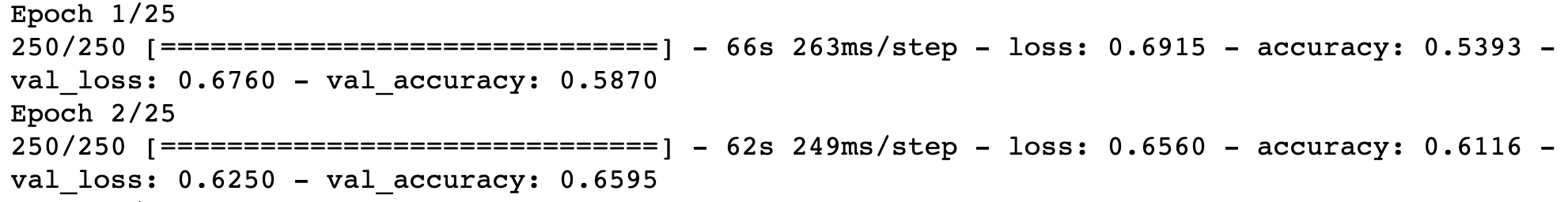
You should see something like this as your convolutional neural network is being trained:
This printed output shows the loss function's value and the model's accuracy in each epoch (or iteration) of our training process for this convolutional neural network. You should notice that the metrics improve over time.
Once this process has been completed, you have successfully trained your convolutional neural network. We can now make predictions using the trained model.
Making Predictions With Our Convolutional Neural Network
It's now time to make predictions using our fully trained convolutional neural network.
We'll be making use of the image module from the preprocessing module within keras to do this.
You may recall that we have already used the ImageDataGenerator class from within this module earlier in this tutorial. However, we didn't actually import the entire image module, so we'll do that now with the following command:
from tensorflow.keras.preprocessing import imageThe next thing we need to do is load the images we're using to make predictions into our Python script. We'll be making predictions on two images: one image that contains a cat and one image that contains a dog.
Both images live within the predictions folder of our current working directory. Their file names are cat_or_dog_1.jpg and cat_or_dog_2.jpg
To load these images into our Python script, we need to use the load_img function from the image module. This function accepts two parameters:
- The filepath of the image you'd like to load in (including the file extension).
- The target size that you'd like to resize the image to. This is a very important parameter since the image must be resized to the same dimensions as the training data. Recall that we had previously resized the training data to be
64x64, so we will specifytarget_size = (64, 64).
Here are the Python statements to load our two images into the program:
test_image_1 = image.load_img('predictions/cat_or_dog_1.jpg', target_size = (64, 64))

test_image_2 = image.load_img('predictions/cat_or_dog_2.jpg', target_size = (64, 64))
These images now need to be transformed slightly before they can be passed into our predict method. As discussed previously in this tutorial, the predict method accepts a two-dimensional NumPy array of pixel colors.
Fortunately, there is a function called img_to_array with the image module that makes it easy to perform this transformation.
Here are the commands to do this:
test_image_1 = image.img_to_array(test_image_1)

test_image_2 = image.img_to_array(test_image_2)
The last step of perdition preprocessing that must be performed is to batch our test data.
Remember that we specified batch_size = 32 in our flow_from_directory function earlier in this tutorial? This means that our training data was grouped into batches of size 32 when the model was trained. We must match this batch size to calculate predictions on our test data.
We will use NumPy's expand_dims function to do this, which will artificially expand the dimensions of our photo's data. Here are the commands to do this:
test_image_1 = np.expand_dims(test_image_1, axis = 0)

test_image_2 = np.expand_dims(test_image_2, axis = 0)
That concludes the preprocessing of our prediction data. We can now use our convolutional neural network to make a prediction about whether an image contains a cat or a dog!
As with most machine learning models, we can calculate predictions using the aptly-named predict method called on our cnn object. Here's how to do this for the first image;
print(cnn.predict(test_image_1))This outputs:
[[0.9996136]]Similarly, here's how we can make a prediction for the second image:
print(cnn.predict(test_image_2))This outputs:
[[0.4850491]]These predictions are meaningless without knowing whether 1 and 0 are assigned to cats or dogs by our convolutional neural network.
Fortunately, determining which number corresponds to each animal is simple.
The training_set variable that we created earlier in this tutorial contains an attribute called class_indices that is a dictionary with keys and values showing which number corresponds to each animal.
You can reference the dictionary with training_set.class_indices. Here's the dictionary for our convolutional neural network:
{'cats': 0, 'dogs': 1}With this information, you can now recognize that our model believes the first image is a dog (since its predicted value is greater than 0.5) and the second image is a cat (since its predicted values is less than 0.5).
Both predictions are correct! It is also worth noting that each numerical output from our convolutional neural network can be interpreted as the probability that an image contains a dog.
If you'd prefer to make categorical predictions (cat or dog) instead of numerical predictions, you can do this by adding the following if statements to the end of your Python script:
#Making categorial predictions

result_1 = cnn.predict(test_image_1)

result_2 = cnn.predict(test_image_2)

if (result_1 >= 0.5):

    result_1 = 'dog'

else:

    result_1 = 'cat'


if (result_2 >= 0.5):

    result_2 = 'dog'

else:

    result_2 = 'cat'


print(result_1)

print(result_2)
The Full Code For This Tutorial
You can view the full code for this tutorial in this GitHub repository. It is also pasted below for your reference:
#Import the necessary libraries

import numpy as np

import pandas as pd

import tensorflow as tf

from tensorflow.keras.preprocessing.image import ImageDataGenerator

#Preprocessing the training set

training_generator = ImageDataGenerator(

                        rescale = 1/255,

                        shear_range = 0.2,

                        zoom_range = 0.2,

                        horizontal_flip = True)

training_set = training_generator.flow_from_directory('training_data',

                                                 target_size = (64, 64),

                                                 batch_size = 32,

                                                 class_mode = 'binary')

#Preprocessing the test set

test_generator = ImageDataGenerator(rescale = 1./255)

test_set = test_generator.flow_from_directory('test_data',

                                            target_size = (64, 64),

                                            batch_size = 32,

                                            class_mode = 'binary')

#Building the artificial neural network

cnn = tf.keras.models.Sequential()

#Adding the convolutional layer

cnn.add(tf.keras.layers.Conv2D(filters=32, kernel_size=3, activation='relu', input_shape=[64, 64, 3]))

#Adding our max pooling layer

cnn.add(tf.keras.layers.MaxPool2D(pool_size=2, strides=2))

#Adding another convolutional layer and max pooling layer

cnn.add(tf.keras.layers.Conv2D(filters=32, kernel_size=3, activation='relu'))

cnn.add(tf.keras.layers.MaxPool2D(pool_size=2, strides=2))

#Adding Our flattening Layer

cnn.add(tf.keras.layers.Flatten())

#Adding our full connection layer

cnn.add(tf.keras.layers.Dense(units=128, activation='sigmoid'))

#Adding our output layer

cnn.add(tf.keras.layers.Dense(units=1, activation='sigmoid'))

#Compiling our convolutional neural network

cnn.compile(optimizer = 'adam', loss = 'binary_crossentropy', metrics = ['accuracy'])

#Training our convolutional neural network

cnn.fit(x = training_set, validation_data = test_set, epochs = 25)

#Prediction preprocessing

from tensorflow.keras.preprocessing import image

test_image_1 = image.load_img('predictions/cat_or_dog_1.jpg', target_size = (64, 64))

test_image_2 = image.load_img('predictions/cat_or_dog_2.jpg', target_size = (64, 64))

test_image_1 = image.img_to_array(test_image_1)

test_image_2 = image.img_to_array(test_image_2)

test_image_1 = np.expand_dims(test_image_1, axis = 0)

test_image_2 = np.expand_dims(test_image_2, axis = 0)

#Making predictions on our two isolated images

print(cnn.predict(test_image_1))

print(cnn.predict(test_image_2))

#Determining which number corresponds to each animal

Training_set.class_indices

#Making categorial predictions

result_1 = cnn.predict(test_image_1)

result_2 = cnn.predict(test_image_2)

if (result_1 >= 0.5):

    result_1 = 'dog'

else:

    result_1 = 'cat'


if (result_2 >= 0.5):

    result_2 = 'dog'

else:

    result_2 = 'cat'


print(result_1)

print(result_2)
Final Thoughts
This tutorial taught you how to build your first convolutional neural network from scratch.
Here is a brief summary of what we discussed in this tutorial:
- How to load image data sets into a Python script using the
ImageDataGeneratorclass fromkeras - How to apply image augmentation techniques to training data (but not the test data!) that will be used in a convolutional neural network
- How to initialize a convolutional neural network using the
Sequentialclass from themodelsmodule ofkeras - How to add convolutional layers to the CNN using the
Conv2Dclass - How to add max pooling layers to the CNN using the
MaxPool2Dclass - How to add a flattening step using the
Flattenmethod that transforms the output of the artificial neural network into a one-dimensional array that can be used as the input of the ANN in the full connection step - How to add a full connection layer and an output layer to a convolutional neural network using the
Denseclass - How to train a convolutional neural network using the
fitmethod - How to deploy a convolutional neural network on real images to make predictions about whether an image contains a cat or a dog.
- How to modify your Python script so that it makes categorical predictions instead of numerical predictions