How To Build And Train An Artificial Neural Network

Hey - Nick here! This page is a free excerpt from my $199 course Python for Finance, which is 50% off for the next 50 students.

If you want the full course, click here to sign up.

So far in this course, we have explored many of the theoretical concepts that one must understand before building your first neural network.

These concepts include:

The structure of a neural network
The role of neurons, activation functions, and gradient descent in deep learning
How neural networks work and how they are trained

It's now time to move on to more practical material. More specifically, this tutorial will teach you how to build and train your first artificial neural network.

You can skip to a specific section of this Python deep learning tutorial using the table of contents below:

The Imports We Will Need For This Tutorial
Importing Our Data Set Into Our Python Script
Data Preprocessing
Working With Categorical Data in Machine Learning
Splitting The Data Set Into Training Data and Test Data
Feature Scaling Our Data Set For Deep Learning
Building The Artificial Neural Network
Training The Artificial Neural Network
- Compiling The Neural Network
- Training The Model On Our Test Data
Making Predictions With Our Artificial Neural Network
Measuring The Performance Of The Artificial Neural Network Using The Test Data
The Full Code For This Tutorial
Final Thoughts

The Imports We Will Need For This Tutorial

To start, navigate to the same folder that you moved the data set into during the last tutorial. Then open a Jupyter Notebook.

The first thing we'll do inside our Jupyter Notebook is import various open-source libraries that we'll use throughout our Python script, including NumPy, matplotlib, pandas, and (most importantly) TensorFlow. Run the following import statements to start your script:

import numpy as np

import pandas as pd

import matplotlib.pyplot as plt

import tensorflow as tf

Note that if you receive the following error message for TensorFlow, then you will need to install TensorFlow on your local machine.

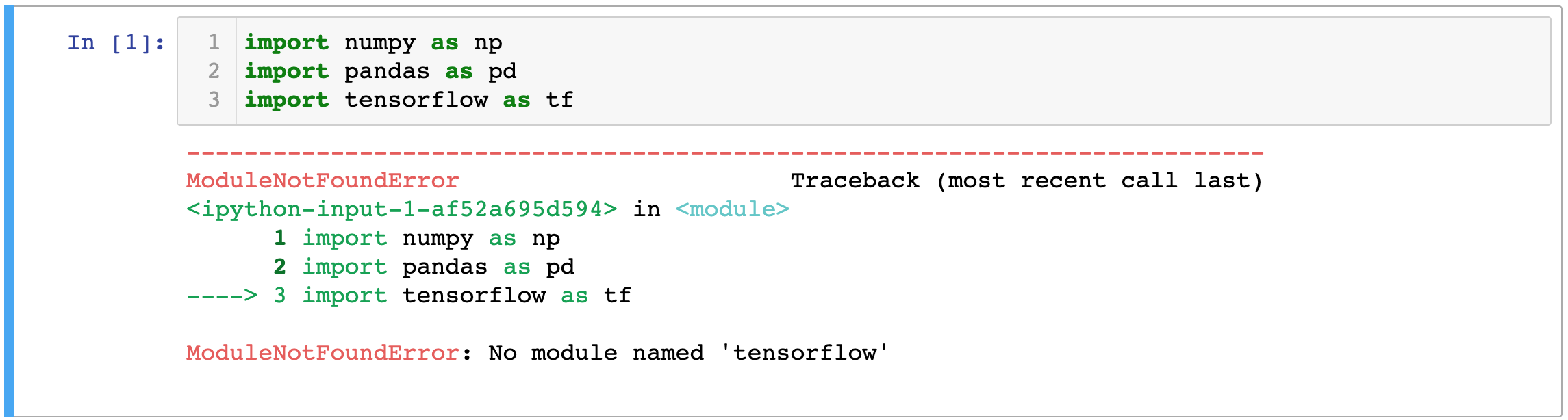
An error message received when trying to import TensorFlow

If this happens, install TensorFlow by running the follow command in your Terminal:

pip3 install tensorflow

This command installs the latest stable release of TensorFlow. At the time of this writing, that is TensorFlow Core v2.2.0. If you're unsure which release of TensorFlow you're working with, you can access this information using the tf.__version__ attribute like this:

TensorFlow version 2.2.0

One last thing - note that TensorFlow is a very large module, so the import tensorflow as tf statement will take longer than other imports you're familiar with (such as import pandas as pd or import numpy as np).

Importing Our Data Set Into Our Python Script

The next thing we'll do is import our data set into the Python script we're working on. More specifically, we will store the data set in a pandas DataFrame using the read_csv method, like this:

raw_data = pd.read_csv('bank_data.csv')

If you print this raw_data variable inside of your Jupyter Notebook, it should look something like this:

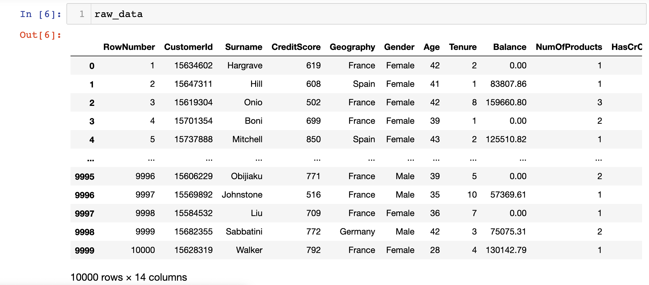
The raw data set we will be using in this tutorial

Now let's move on to performing some preprocessing on our bank customer data set.

Data Preprocessing

If you look at this data set, you will notice that the first three columns are RowNumber, CustomerId, and Surname. Neither of these features will be useful in predicting customer churn for the bank. Accordingly, we should remove them from the data set.

With that in mind, we can store all of the features of this data set in a variable called x_data with the following statement:

x_data = raw_data.iloc[:, 3:-1].values

Similarly, we can store the labels of this data set in a variable called y_data with the following statement:

y_data = raw_data.iloc[:, -1].values

Both the x_data and y_data variables are NumPy arrays that contain the x-values (also called our features) and the y-data (also called our labels) that we'll use to train our artificial neural network later.

Before we can train our data, we must first make some modifications to the categorical data within our data set.

Working With Categorical Data in Machine Learning

If you print the raw_data.columns attribute, you will generate the following output:

Index(['RowNumber', 'CustomerId', 'Surname', 'CreditScore', 'Geography',

       'Gender', 'Age', 'Tenure', 'Balance', 'NumOfProducts', 'HasCrCard',

       'IsActiveMember', 'EstimatedSalary', 'Exited'],

      dtype='object')

There are two categorical variables in the data set: Gender and Geography. We must massage these variables slightly to make them easier to interpret for our artificial neural network.

First, let's identify which columns need to be modified by printing the x_data variable within our Jupyter Notebook:

Our original x_data variable

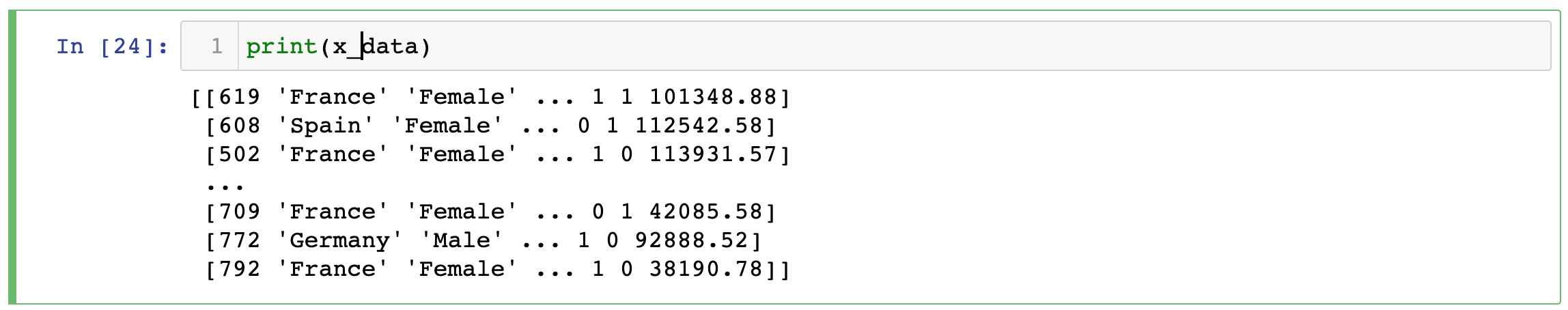
As you can see, the Geography and Gender columns are the second and third columns within the NumPy array. They have indices of 1 and 2, respectively.

These variables need to be modified differently because in the case of Gender, there is a relationship between the two categories. Knowing that someone is Male tells us that they are not Female, and vice versa. There is no such logical relationship for the Geography column, which has many more possible values.

Let's start by modifying the Gender column. We will use the LabelEncoder class from scikit-learn to do this.

To start, import the LabelEncoder class from the preprocessing module of scikit-learn with the following statement:

from sklearn.preprocessing import LabelEncoder

Then create an instance of the LabelEncoder class and assign it to the variable name label_encoder:

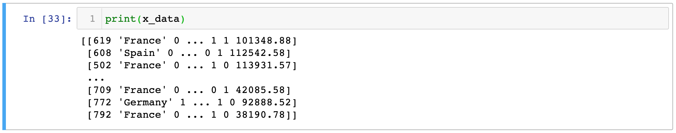
label_encoder = LabelEncoder()

Now we can encode the data within the Gender column with the following statement:

x_data[:, 2] = label_encoder.fit_transform(x_data[:, 2])

Let's print the x_data variable again to see how this code has modified our data set.

Our x_data variable with the Gender column modified

As you can see, all Female data points have been re-assigned a value of 0. Similarly, all Male data points have been assigned a value of 1.

Let's perform similar preprocessing on the Geography column. More specifically, we will use a preprocessing technique called One Hot Encoding, which will create a new column for every value in the Geography column.

If the old column contained that specific value, then the new column will contain 1. Otherwise, the column will contain 0.

Here is the code to do this:

from sklearn.compose import ColumnTransformer

from sklearn.preprocessing import OneHotEncoder

transformer = ColumnTransformer(transformers = [('encoder', OneHotEncoder(), [1])], remainder = 'passthrough')

x_data = np.array(transformer.fit_transform(x_data))

Let's print the modified x_data variable to see how this has modified the data set.

Our x_data variable with the Geography column modified

You might be wondering where our original values for the CreditScore column have gone! Well, whenever you perform one hot encoding using scikit-learn, the new columns are always moved to the front of the NumPy array.

If you've never performed one hot encoding before, here's how to interpret the new columns:

If the original Geography column had a value of France, then the first three columns will contains [1, 0, 0]
If the original Geography column had a value of Germany, then the first three columns will contains [0, 1, 0]
If the original Geography column had a value of France, then the first three columns will contains [0, 0, 1]

Our data preprocessing is now finished. It's time to split our data set into training data and test data.

Splitting The Data Set Into Training Data and Test Data

Machine learning practitioners almost always use scikit-learn's built-in train_test_split function to split their data set into training data and test data.

To start, let's import this function into our Python script:

from sklearn.model_selection import train_test_split

The train_test_split function returns a Python list of length 4 with the following items:

The x training data
The x test data
The y training data
The y test data

train_test_split is typically combined with list unpacking to easily create 4 new variables that store each of the list's items. As an example, here's how we'll create our training and test data using a test_size parameter of 0.3 (which simply means that the test data will be 30% of the observations of the original data set).

x_training_data, x_test_data, y_training_data, y_test_data = train_test_split(x_data, y_data, test_size = 0.3)

Feature Scaling Our Data Set For Deep Learning

The next thing we need to do is feature scaling, which is the process of modifying our independent variables so that they are all roughly the same size.

Feature scaling is absolutely critical for deep learning. While many statistical methods benefit from feature scaling, it is actually required for deep learning.

We'll apply feature scaling to every feature of our data set because of this. To start, import the StandardScaler class from scikit-learn and create an instance of this class. Assign the class instance to a variable named scaler:

from sklearn.preprocessing import StandardScaler

scaler = StandardScaler()

Next, execute the fit_transform method from our scaler object to apply feature scaling to both our training data and test data with the following statements:

x_training_data = scaler.fit_transform(x_training_data)

x_test_data = scaler.fit_transform(x_test_data)

Building The Artificial Neural Network

We will follow four broad steps to build our artificial neural network:

Initializing the Artificial Neural Network
Adding The Input Layer & The First Hidden Layer
Adding The Second Hidden Layer
Adding The Output Layer

Let's go through each of these steps one-by-one.

Initializing the Artificial Neural Network

To start, let's initialize our artificial neural network and assign it to a variable named ann:

ann = tf.keras.models.Sequential()

Let's break down what's happening here:

We're creating an instance of the Sequential class
The Sequential class lives within the models module of the keras library
Since TensorFlow 2.0, Keras is now a part of TensorFlow, so the Keras package must be called from the tf variable we created earlier in our Python script

All of this code serves to create a "blank" artificial neural network.

Adding The Input Layer & The First Hidden Layer

Now it's time to add our input layer and our first hidden layer.

Let's start by discussing the input layer. No action is required here. Neural network input layers do not need to actually be created by the engineer building the network.

Why is this?

Well, if you think back to our discussion of input layers, remember that they are entirely decided by the data set that the model is trained on. We do not need to specify our input layer because of this.

With that in mind, we can move on to adding the hidden layer.

Layers can be added to a TensorFlow neural network using the add method. To start, call the add method on our ann variable without passing in any parameters:

ann.add()

Now what do we need to pass in to create our hidden layer?

keras contains a module called layers that contains pre-built classes for the different types of neural network layers you might want to add to your model. In this case, we will be adding the a Dense layer. You can create a Dense layer with the following statement:

tf.keras.layers.Dense()

This Dense class requires a single parameter - the number of neurons you'd like to include in the new layer of your neural net. This is perhaps the most commonly-asked question in deep learning and is worth taking a moment to consider.

Unfortunately, there is no rule of thumb to help decide the number of neurons to include in your hidden layers. This is part of the "art" of deep learning and not the "science" of deep learning.

Often the best way to decide the appropriate number of neurons to include is experimentation. Try different numbers of neurons and see which seems to have the best predictive capacity. For the purpose of this tutorial, we'll use 6.

This means that our final statement to add our hidden layer becomes:

ann.add(tf.keras.layers.Dense(units=6))

Another parameter that we might want to change (although we do not need to change it) is the neural network's activation function. By default, there is no activation function applied in the Dense layer. This means that the weighted sum of input values is simply passed on to the next layer of the network.

In our case, we'll be using the Rectified Linear Unit (ReLU) activation function, which can be added to this layer of our ANN by modifying the command as follows:

ann.add(tf.keras.layers.Dense(units = 6, activation = 'relu'))

We have now added our first hidden layer!

In practitioner's terms, this means that we have created a "shallow" neural network. Let's improve this to a "deep" neural network by adding another hidden layer next.

Adding The Second Hidden Layer

Adding a second hidden layer follows the exact same process as the original hidden layer. Said differently, the add method does not need to be used specifically for the first hidden layer of a neural network!

Let's add another hidden layer with 6 units that has a ReLU activation function:

ann.add(tf.keras.layers.Dense(units = 6, activation = 'relu'))

Our neural network is now composed of an input layer and two hidden layers. In the next section, we'll add our output layer and our model will be fully built.

Adding The Output Layer

Like the hidden layers that we added earlier in this tutorial, we can add our output layer to the neural network with the add function. However, we'll need to make several modifications to the statement we used previously.

First of all, let's discuss how many units our output layer should have. Since we are predicting binary data (whether or not a bank customer has churned), we can specify units = 1. If we were working with an output variable that had more dimensions, however, that number would need to increase.

As an example, imagine we were trying to solve a classification problem with 3 categories: A, B, and C. You would want three neurons in the output layer. The different categories would be represented by the following values in those neurons:

A: (1, 0, 0)
B: (0, 1, 0)
C: (0, 0, 1)

This example only has two categories (churned or not churned), so an output layer with units = 1 is sufficient.

The other thing we need to change is our activation function. We want to estimate the probability that a bank customer will churn. Because of this, the Sigmoid function is an excellent choice for oru output layer's activation function.

Let's take these two changes into account and add our output layer to the neural network:

ann.add(tf.keras.layers.Dense(units = 1, activation = 'sigmoid'))

As you can see, building an artificial neural network with TensorFlow is much easier than you'd imagine. We did it in four lines of code:

#Building The Neural Network

ann = tf.keras.models.Sequential()

ann.add(tf.keras.layers.Dense(units = 6, activation = 'relu')) #First hidden layer

ann.add(tf.keras.layers.Dense(units = 6, activation = 'relu')) #Second hidden layer

ann.add(tf.keras.layers.Dense(units = 1, activation = 'sigmoid')) #Output layer

Training The Artificial Neural Network

Our artificial neural network has been built. Now it's time to train the model using the training data we created earlier in this tutorial. This process is divided into two steps:

Compiling the neural network
Training the neural network using our training data

Compiling The Neural Network

In deep learning, compilation is a step that transforms the simple sequence of layers that we previously defined into a highly efficient series of matrix transformations. You can interpret compilation as a precompute step that makes it possible for the computer to train the model.

TensorFlow allows us to compile neural networks using its compile function, which requires three parameters:

The optimizer
The cost function
The metrics parameter

Let's first create a blank compile method call that includes these three metrics (without specifying them yet):

ann.compile(optimizer = , loss = , metrics = )

Let's start by selecting our optimizer. We will be using the Adam optimizer, which is a highly performant stochastic gradient descent algorithm descent specifically for training deep neural networks.

Our compile method becomes:

ann.compile(optimizer = 'adam', loss = , metrics = )

Our loss function will be binary_crossentropy. We do not actually have any choice when it comes to our loss function - whenever you are training a binary classification deep learning model, you must use this loss function. If you were training a deep learning neural network to predict multiple categories, you would instead use categorical_crossentropy.

Our compile method is now:

ann.compile(optimizer = 'adam', loss = 'binary_crossentropy', metrics = )

The last parameter we need to specify is metrics, which is a list of metrics you will use to measure the performance of your model. For simplicity's sake, we will only be using one metric: accuracy.

This metric must be passed in as a list (even if we're only using a single metric), so our compile statement becomes:

ann.compile(optimizer = 'adam', loss = 'binary_crossentropy', metrics = ['accuracy'])

Let's move on to training our artificial neural network.

Training The Model On Our Test Data

As with most machine learning models, artificial neural networks built with the TensorFlow library are trained using the fit method.

The fit method takes 4 parameters:

The x values of the training data
The y values of the training data
The batch_size - this is because we do not train the model on the data's observations one-by-one, but instead in batches. This is more performant. Most machine learning engineers use a batch_size of 32 by default.
The number of epochs - this represents the number of times the artificial neural network will pass over the entire data set during its training phase. We will be using an epochs value of 100.

Adding all of this together, our fit statement becomes:

ann.fit(x_training_data, y_training_data, batch_size = 32, epochs = 100)

When you run this statement, you will see 20 outputs generated one-by-one that print the accuracy of the model for each iteration of the neural network. The accuracy of the neural network stabilizes around 0.86.

Making Predictions With Our Artificial Neural Network

Now that our artificial neural network has been trained, we can use it to make predictions using specified data points. We do this using the predict method.

Before we start, you should note that anything passed into a predict method called on an artificial neural network built using TensorFlow needs to be a two-dimensional array. This necessitates the use of double square brackets, like this:

ann.predict([[]])

With this in mind, let's predict whether or not a bank customer will churn if they have the following characteristics:

Geography: France
Credit Score: 555
Gender: Male
Age: 52 years old
Tenure: 4 years
Balance: $75000
Number of Products: 3
Does this customer have a credit card ? No
Is this customer an Active Member: Yes
Estimated Salary: $ 65000

Here's the code to do this:

ann.predict([[1, 0, 0, 555, 1, 52, 4, 75000, 3, 0, 1, 65000]])

Recall that the encoding for a Geography of France is (1, 0, 0) and the encoding for a Gender of Male is 1. Most of the other values in this array should be fairly straightforward.

There is still a problem with this predict method. Namely, the features we're making predictions with haven't been standardized. You can fix this using the scaler.transform method, which uses the StandardScaler instance that we created earlier in this tutorial to standardize the data:

ann.predict(scaler.transform([[1, 0, 0, 555, 1, 52, 4, 75000, 3, 0, 1, 65000]]))

This returns:

array([[0.9715825]], dtype=float32)

This indicates that our model predicts a 97% chance that this customer will churn from the bank.

If you want a more simple "yes or no" representation of whether a customer will churn, you can modify the code as follows:

ann.predict(scaler.transform([[1, 0, 0, 555, 1, 52, 4, 75000, 3, 0, 1, 65000]])) > 0.5

This returns a boolean value of True if the customer's probability of churning is greater than 50% and a boolean value of False otherwise. You can change the 0.5 threshold to any number you'd like, but 0.5 is a good base case.

Measuring The Performance Of The Artificial Neural Network Using The Test Data

The last thing we'll do in this tutorial is measure the performance of our artificial neural network on our test data.

To start, let's generate an array of boolean values that predicts whether every customer in our test data will churn or not. We will assign this array to a variable called predictions.

predictions = ann.predict(x_test_data) > 0.5

We can now use this predictions variable to generate a confusion matrix, which is a common tool used to measure the performance of machine learning models. We'll need to import the confusion_matrix function from scikit-learn to do this:

from sklearn.metrics import confusion_matrix

Now you can generate the confusion matrix with the following statement:

confusion_matrix(y_test_data, predictions)

This generates:

array([[2297,  125],

       [ 288,  290]])

You might also want to calculate the accuracy of our model, which is the percent of predictions that were correct. scikit-learn has a built-in function called accuracy_score to calculate this, which you can import with the following statement:

from sklearn.metrics import accuracy_score

You can now calculate an accuracy score as follows:

accuracy_score(y_test_data, predictions)