Recommendation systems allow a user to receive recommendations from a database based on their prior activity in that database.

Companies like Facebook, Netflix, and Amazon use recommendation systems to increase their profits and delight their customers.

In this tutorial, you will learn how to build your first Python recommendations systems from scratch.

Table of Contents

You can skip to a specific section of this Python recommendation systems tutorial using the table of contents below:

• The Problem We Will Be Solving In This Tutorial
• The Libraries We Need For This Tutorial
• Importing Our Movie Database

• Exploratory Data Analysis

  • Calculating The Movies With The Highest Average Rating
  • Calculating The Movies With The Most Ratings
  • Visualizing the Ratings in Our Data Set
  • The Relationship Between Average Rating and Number of Ratings
• How to Build a Movie Recommendation System
• The Full Code For This Tutorial
• Final Thoughts

The Problem We Will Be Solving In This Tutorial

Netflix operates one of the world's most popular recommendation systems.

Their machine learning algorithm suggests new movies and TV shows for you to watch based on the previous Netflix content that you have consumed.

We will solve a similar problem in this tutorial. Namely, we will build a basic recommendation system that suggests movies from a movie database that are most similar to a particular movie from that same database.

To start, we'll need to import some open-source Python libraries. We'll also import the movie database later in this tutorial.

The Libraries We Need For This Tutorial

This tutorial will make use of a number of open-source Python libraries, including NumPy, pandas, and matplotlib. We'll import these libraries now.

To start, open a Jupyter Notebook in the directory you'd like to work in. Here are the imports that we will start our Python script with:

#Data imports

import pandas as pd

import numpy as np

#Visualization imports

import matplotlib.pyplot as plt

import seaborn as sns

%matplotlib inline

Now that our imports have been executed, we can move on to importing our movie database.

Importing Our Movie Database

The first thing you'll need to do is download the files that contain our data set. Click the following three links to download a version of each file to your Downloads folder:

• Movie database download 1
• Movie database download 2
• Movie database download 3

This will download three files named:

• Movie_Id_Titles
• u.data
• u.item

Move these files into the directory that you'd like to work in for this tutorial. This needs to be the same folder that you opened your Jupyter Notebook in earlier.

Then, you'll need to import the data into a pandas DataFrame.

The actual data for our movie database lies within the u.data file. Here is the command required to import the data into a DataFrame:

raw_data = pd.read_csv('u.data', sep = '\t', names = ['user_id', 'item_id', 'rating', 'timestamp'])

You will notice that this DataFrame has four columns and none of them contain the title of the movie. This data lies in a separate that we downloaded previously named Movie_Id_Titles. You will need to import this data and merge it with our existing raw_data DataFrame before proceeding.

First, let's import the movie title data:

movie_titles_data = pd.read_csv('Movie_Id_Titles')

Now let's merge the two DataFrames together into one DataFrame by merging them on the item_id column:

merged_data = pd.merge(raw_data, movie_titles_data, on='item_id')

You can get a sense of what the new DataFrame contains by running merged_data.columns, which returns:

Index(['user_id', 'item_id', 'rating', 'timestamp', 'title'], dtype='object')

Let's learn more about this data set by performing some exploratory data analysis.

Exploratory Data Analysis

Exploratory data analysis is the process of learning more about a data set by calculating aggregate statistics or creating visualizations. Let's dig in to our merged movies data set before building our recommendation system later in this tutorial.

Calculating The Movies With The Highest Average Rating

For every movie in our data set, there are a number of different ratings that are submitted by the different users of the database.

Let's start by calculating the average rating for every movie in the database with the following command:

merged_data.groupby('title')['rating'].mean().sort_values(ascending = False)

This will return a pandas Series that orders the movies from the highest average rating to the lowest average rating. It will look something like this:

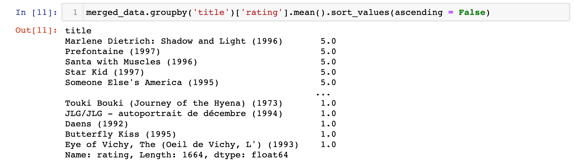
Keep in mind that this does not account for how many ratings each movie has. It is possible that movies with an "average" rating of 5.0 only have a single rating. The same applies for movies with an "average" rating of 1.0.

We'll solve this problem in the next section by identifying the movies in our data set that have the most ratings.

Calculating The Movies With The Most Ratings

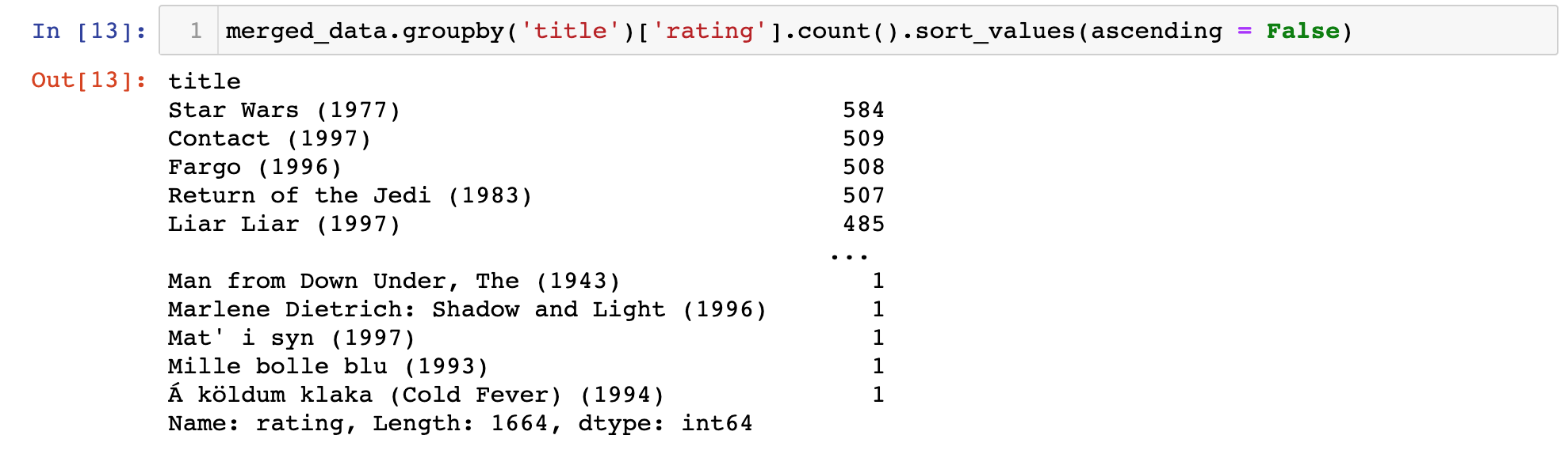
You can list the movies in order of their number of ratings with the following command:

This generates the following output:

Visualizing the Ratings in Our Data Set

Now we will visualize the distribution of movie ratings in our data set.

It will be helpful to store our ratings in a simpler data structure first.

Accordingly, let's quickly create a pandas DataFrame that contains the average rating and the number of ratings for every movie in the data set.

Let's start the DataFrame with just the average rating by movie with the following statement:

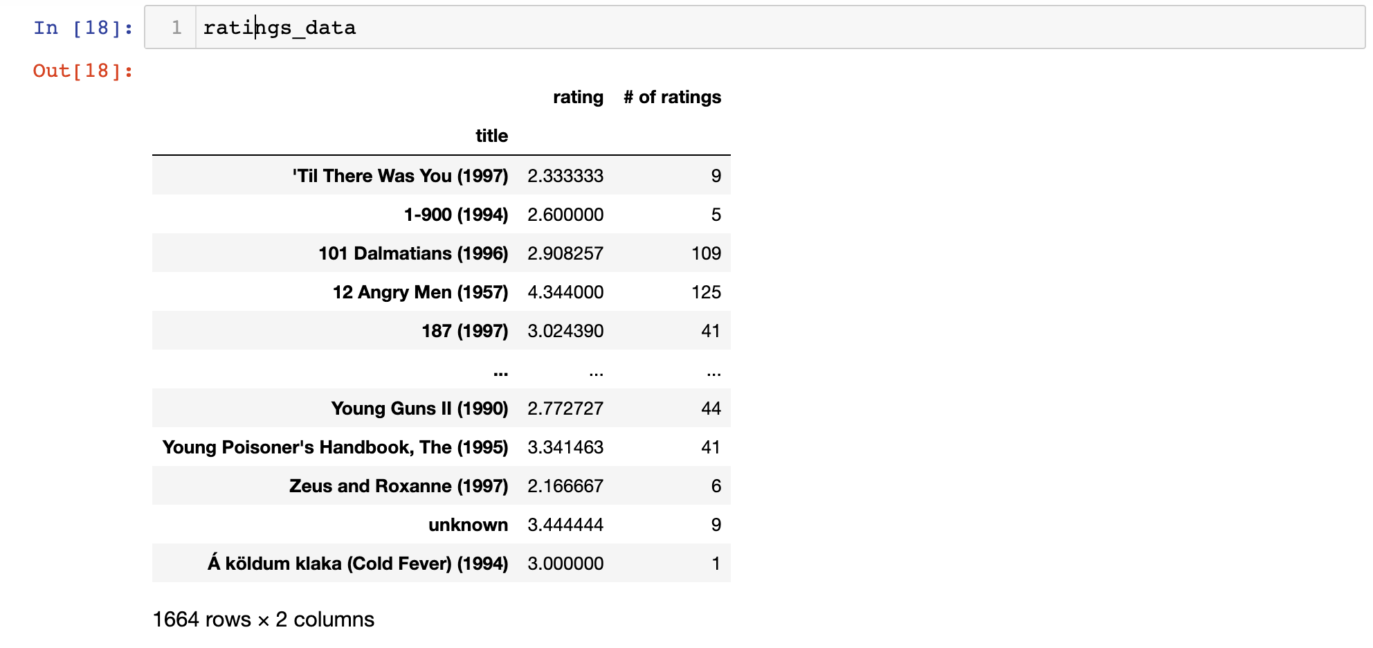
ratings_data = pd.DataFrame(merged_data.groupby('title')['rating'].mean())

Next let's add another column to this DataFrame that contains the number of ratings for every movie in the data set:

ratings_data['# of ratings'] = merged_data.groupby('title')['rating'].count()

Here's what this new ratings_data DataFrame looks like:

We can now use this DataFrame to create some nice visualizations.

First, let's visualize the distribution of number of ratings by movie using seaborn's distplot function:

sns.distplot(ratings_data['# of ratings'])

Here is the histogram that this generates:

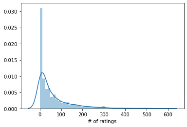
As you can see, most movies seem to have either 0 ratings or 1 rating. This makes sense - very few movies have the mass appeal to receive many ratings from watchers.

Let's create a similar visualization for the actual rating assign to the movies:

sns.distplot(ratings_data['rating'])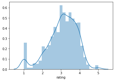

As you can tell, most movies seem to be distributed around a rating of 3 or so, with peaks at 1, 2, 4, and 5 - which are presumably movies with only one rating.

The Relationship Between Average Rating and Number of Ratings

Let's create one last visualization that explores the relationship between a movie's average rating and its number of ratings.

The seaborn jointplot is a nice visualization for this. We can create our jointplot with the following command:

sns.jointplot(x = ratings_data['rating'], y = ratings_data['# of ratings'])

This generates the following plot:

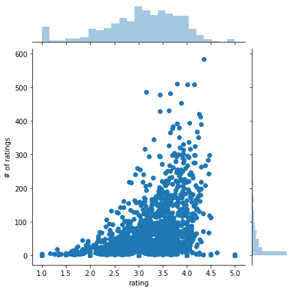
It seems like there seems to be some positive relationship between the number of ratings and the average rating. Said differently, movies with high average ratings tend to have more ratings, and vice versa.

We have now spent some time on exploratory data analysis, which ensures that we have a good sense of the structure of our data before building our recommendation system.

Let's move on to determining the similarity of two movies in the next section.

How to Build a Movie Recommendation System

Our recommendation system functions based on the similarities between movies. More specifically, it will recommend movies to you that other users with similar taste have enjoyed.

To demonstrate this, we'll select two movies from the data set:

• Toy Story (1995)
• Returns of the Jedi (1983)

The first thing we need to do is create matrices that contain the user ratings for each movie in the data set. These movie matrices will allow you to see how each user rated every movie in the data set.

Let's create these user rating matrices with the following code:

ratings_matrix = merged_data.pivot_table(index='user_id',columns='title',values='rating')

star_wars_user_ratings = ratings_matrix['Return of the Jedi (1983)']

toy_story_user_ratings = ratings_matrix['Toy Story (1995)']

Let's examine what's stored in the toy_story_user_ratings and star_wars_user_ratings variables.

More specifically, here's the command you can use to print the first 5 entries in the toy_story_user_ratings data structure:

toy_story_user_ratings.head(5)

This will generate the following:

user_id

0    NaN

1    5.0

2    NaN

3    4.0

4    NaN

This data structure is a pandas Series that contains the rating given to the Toy Story (1995) movie. A value of NaN is stored if a specific user has not provided a rating for the Toy Story (1995) movie. The user ID of the user who provided the rating is stored as the index of the Series.

Next, we will use the corrwith method to calculate the correlation between the toy_story_user_ratings and star_wars_user_ratings data sets. This will allow us to see if the movies are similar, since their ratings distribution among users will be highly correlated if so!

Here is the command to calculate the correlation between the two pandas Series:

ratings_matrix.corrwith(toy_story_user_ratings)['Return of the Jedi (1983)']

Let's break down this statement.

First, a pandas Series is created using ratings_matrix.corrwith(toy_story_user_ratings) that shows the correlation of user ratings between the Toy Story (1995) movie and every other movie in the data set.

Next, the specific correlation for Return of the Jedi (1983) is pulled from the data structure by passing in the name of the movie in square brackets.

Here's the correlations between the two movies' user ratings:

0.18709230116786751

The movies are not very similar since they have a low correlation.

Let's try and find a movie that _is _highly similar to the Return of the Jedi (1983) movie. To do this, let's build a pandas DataFrame that stores the correlation of every movie's user ratings with the Return of the Jedi (1983) user ratings.

Here is the command to do this:

correlation_with_star_wars = pd.DataFrame(ratings_matrix.corrwith(star_wars_user_ratings))

correlation_with_star_wars.dropna().sort_values(0, ascending = False).head(15)

There is a lot going on in this command, so let's break it down step-by-step:

• The first line of code creates a pandas DataFrame with a single column that shows the correlation of every movie's user ratings with the user ratings of Return of the Jedi (1983)
• The dropna method removes null values from the DataFrame
• The sort_values method combined with the arguments 0 and ascending = False modifies the DataFrame so the most similar movies are shown at the top
• The head(15) method shows only the 15 entries at the top of the DataFrame

This code will generate the following output:

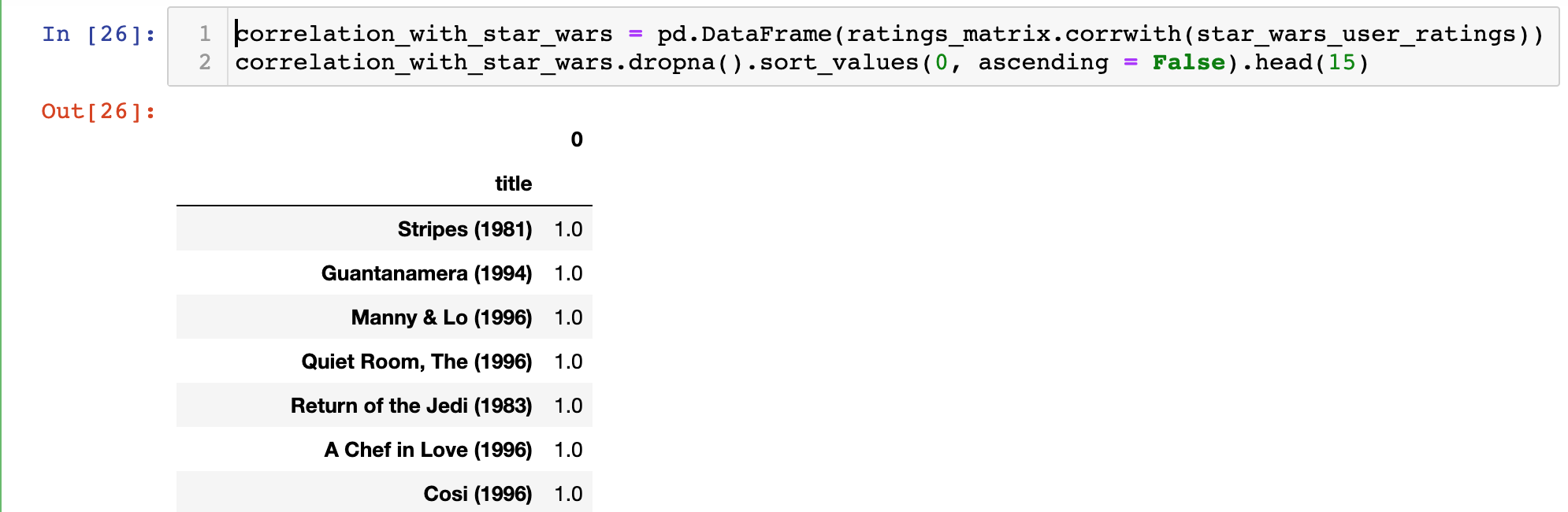
You may notice that some of the results in this DataFrame do not really make sense. Namely, why do so many movies' user ratings have perfect correlations with the user ratings of Return of the Jedi (1983)?

The cause for this anomaly is small sample size bias. Namely, it is likely that these perfectly-correlated movies have only been seen by one person who has also seen Return of the Jedi (1983), and that user happened to give the same rating to both movies.

Fortunately, it is relatively easy to fix this problem. You would simply filter the recommendation system to exclude movies that had less than a certain number of reviews.

Let's filter out movies that have less than 50 reviews to improve the basic recommendation system that we have built in this tutorial so far.

To start this process, we'll want to add the number of ratings from each movie to our ratings_matrix data structure. A simple pandas join operation is perfect for this:

correlation_with_star_wars = correlation_with_star_wars.join(ratings_data['# of ratings'])

Now let's take a moment to update the column and index names of our DataFrame. This will move appropriately reflect the changes we've just made to the data structure:

correlation_with_star_wars.columns = ['Corr. With SW Ratings', '# of Ratings']

correlation_with_star_wars.index.names = ['Movie Title']

The updated data structure should look like this:

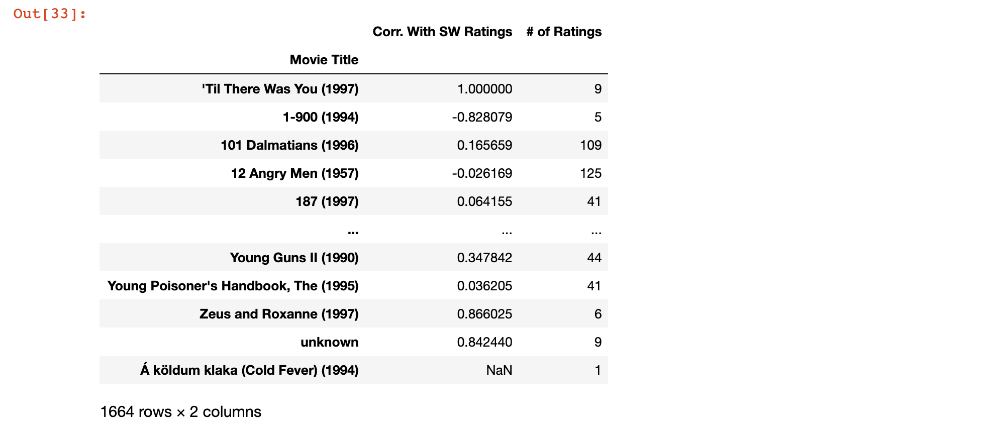
As you can see, the DataFrame now contains the correlation of each movie's ratings with Return of the Jedi (1983) as well as the number of ratings for that specific movie.

What we need to do now is filter out any movies that do not have at least 50 ratings.

As before, we will also sort the DataFrame such that the movies most similar to Return of the Jedi (1983) are displayed at the top.

We'll also use the head method with a parameter of 10 to return the 10 movies that are most similar to Return of the Jedi (1983).

Here the full statement:

correlation_with_star_wars[correlation_with_star_wars['# of Ratings'] > 50].sort_values('Corr. With SW Ratings', ascending = False).head(10)

Here is the output of this statement:

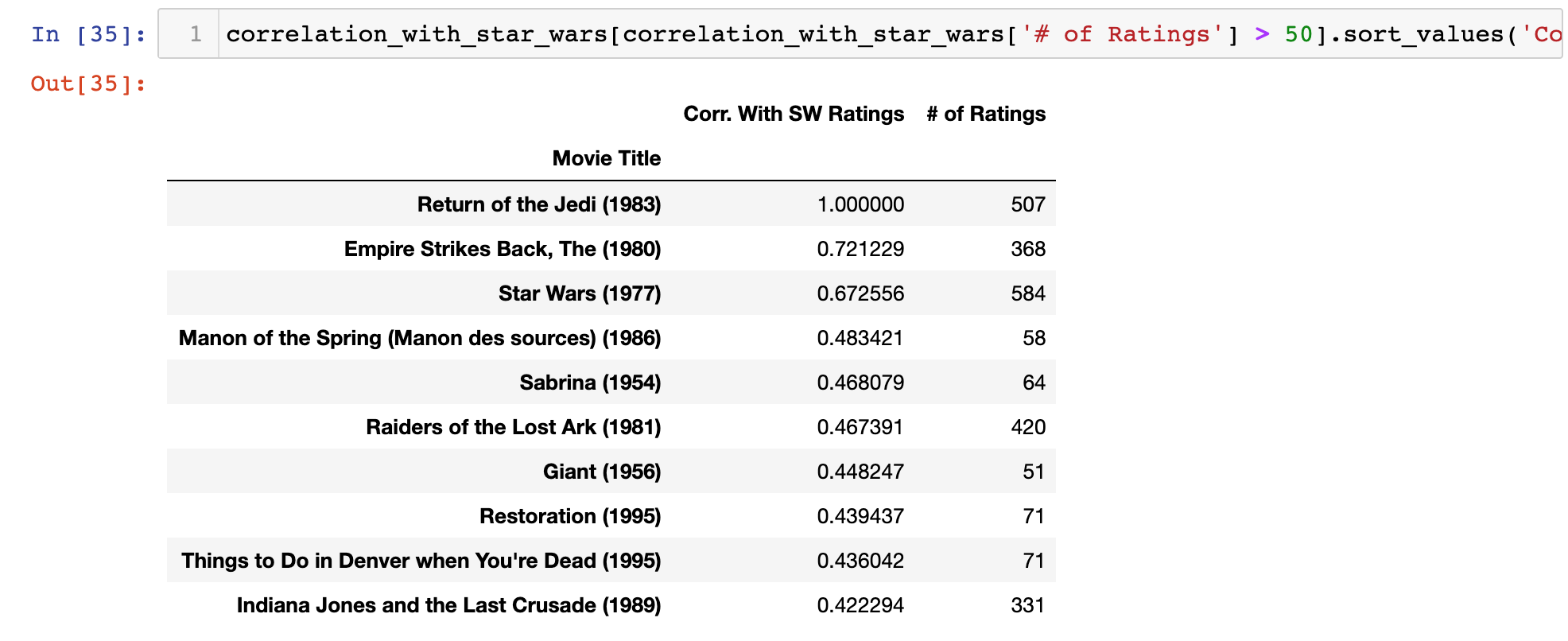
This makes much more sense. As you can see, 3 of the top 10 movies are Star Wars franchise movies. There's also an Indiana Jones movie (Raiders of the Lost Ark (1981)), which has a similar feel to the Star Wars trilogy.

The Full Code For This Tutorial

You can view the full code for this tutorial in this GitHub repository. It is also pasted below for your reference:

#Data imports

import pandas as pd

import numpy as np

#Visualization imports

import matplotlib.pyplot as plt

import seaborn as sns

%matplotlib inline

#Import the data

raw_data = pd.read_csv('u.data', sep = '\t', names = ['user_id', 'item_id', 'rating', 'timestamp'])

movie_titles_data = pd.read_csv('Movie_Id_Titles')

#Merge our two data sources

merged_data = pd.merge(raw_data, movie_titles_data, on='item_id')

merged_data.columns

#Calculate aggregate data

merged_data.groupby('title')['rating'].mean().sort_values(ascending = False)

merged_data.groupby('title')['rating'].count().sort_values(ascending = False)

#Create a DataFrame and add the number of ratings to is using a count method

ratings_data = pd.DataFrame(merged_data.groupby('title')['rating'].mean())

ratings_data['# of ratings'] = merged_data.groupby('title')['rating'].count()

#Make some visualizations

sns.distplot(ratings_data['# of ratings'])

sns.distplot(ratings_data['rating'])

#Create the ratings matrix and get user ratings for `Return of the Jedi (1983)` and `Toy Story (1995)`

ratings_matrix = merged_data.pivot_table(index='user_id',columns='title',values='rating')

star_wars_user_ratings = ratings_matrix['Return of the Jedi (1983)']

toy_story_user_ratings = ratings_matrix['Toy Story (1995)']

ratings_matrix.corrwith(toy_story_user_ratings)['Return of the Jedi (1983)']

#Calculate correlations and source recommendations

correlation_with_star_wars = pd.DataFrame(ratings_matrix.corrwith(star_wars_user_ratings))

correlation_with_star_wars.dropna().sort_values(0, ascending = False).head(15)

#Add the number of ratings and rename columns

correlation_with_star_wars = correlation_with_star_wars.join(ratings_data['# of ratings'])

correlation_with_star_wars.columns = ['Corr. With SW Ratings', '# of Ratings']

correlation_with_star_wars.index.names = ['Movie Title']

#Get new recommendations from movies that have more than 50 ratings

correlation_with_star_wars[correlation_with_star_wars['# of Ratings'] > 50].sort_values('Corr. With SW Ratings', ascending = False).head(10)

Final Thoughts

In this tutorial, you learned how to build your first recommendation system in Python.

Here is a brief summary of what you learned in this tutorial:

• How to perform exploratory data analysis before building a machine learning recommendation system
• How to calculate correlations between user ratings series' using the corrwith method
• How to build a movie recommendation system in Python