Principal Component Analysis in Python - A Step-by-Step Guide

Hey - Nick here! This page is a free excerpt from my new eBook Pragmatic Machine Learning, which teaches you real-world machine learning techniques by guiding you through 9 projects.

Since you're reading my blog, I want to offer you a discount. Click here to buy the book for 70% off now.

Principal component analysis is an unsupervised machine learning technique that is used in exploratory data analysis.

More specifically, data scientists use principal component analysis to transform a data set and determine the factors that most highly influence that data set.

This tutorial will teach you how to perform principal component analysis in Python.

You can skip to a specific section of this Python principal component analysis tutorial using the table of contents below:

The Libraries We Will Be Using in This Tutorial
The Data Set We Will Be Using In This Tutorial
Performing Our First Principal Component Transformation
Visualizing Our Principal Component
What The Heck Is A Principal Component, Anyway?
How to Use Principal Component Analysis in Practice
The Full Code For This Tutorial
Final Thoughts

The Libraries We Will Be Using in This Tutorial

This tutorial will make use of a number of open-source software libraries, including NumPy, pandas, and matplotlib.

Accordingly, we'll start our Python script by adding the following imports:

import pandas as pd

import numpy as np

import matplotlib.pyplot as plt

import seaborn

%matplotlib inline

Let's move on to importing our data set next.

The Data Set We Will Be Using In This Tutorial

Earlier in this course, you learned how to build support vector machines on scikit-learn's built-in breast cancer data set.

We will be using that same data set to learn about principal component analysis in this tutorial.

Let's start importing this data set by loading scikit-learn's load_breast_cancer function.

from sklearn.datasets import load_breast_cancer

When this function is run, it generates the data set. Let's assign the data set to a variable called raw_data:

raw_data = load_breast_cancer()

If you run type(raw_data) to determine what type of data structure our raw_data variable is, it will return sklearn.utils.Bunch. This is a special, built-in data structure that belongs to scikit-learn.

Fortunately, this data type is easy to work with. In fact, it behaves similarly to a normal Python dictionary.

One of the keys of this dictionary-like object is data. We can use this key to transform the data set into a pandas DataFrame with the following statement:

raw_data_frame = pd.DataFrame(raw_data['data'], columns = raw_data['feature_names'])

Let's investigate what features our data set contains by printing raw_data_frame.columns. This generates:

Index(['mean radius', 'mean texture', 'mean perimeter', 'mean area',

       'mean smoothness', 'mean compactness', 'mean concavity',

       'mean concave points', 'mean symmetry', 'mean fractal dimension',

       'radius error', 'texture error', 'perimeter error', 'area error',

       'smoothness error', 'compactness error', 'concavity error',

       'concave points error', 'symmetry error', 'fractal dimension error',

       'worst radius', 'worst texture', 'worst perimeter', 'worst area',

       'worst smoothness', 'worst compactness', 'worst concavity',

       'worst concave points', 'worst symmetry', 'worst fractal dimension'],

      dtype='object')

As you can see, this is a very feature-rich data set.

One last thign to note about our data set is that the variable we're trying to predict - which is whether or not a specific breast cancer tumor is malignant or benign - is held within the raw_data object under the target key.

The target values can be accessed with raw_data['target']. The values will be 1 for malignant tumors and 0 for benign tumors.

Performing Our First Principal Component Transformation

As we saw when we printed our raw_data_frame.columns array, our data set has many features. This makes it difficult to perform exploratory data analysis on the data set using traditional visualization techniques.

To fix this, we need to perform a principal component transformation to transform our data set into one with just two features where each feature is a principal component.

To start, we need to standardize our data set. In machine learning, standardization simply refers to the act of transforming all of the observations in our data set so that each feature is roughly the same size.

We use scikit-learn's StandardScaler class to do this. The first thing we'll need to do is import this class from scikit-learn with the following command:

from sklearn.preprocessing import StandardScaler

Next, we need to create an instance of this class. We'll assign the newly-created StandardScaler object to a variable named data_scaler:

data_scaler = StandardScaler()

We now need to train the data_scaler variable on our raw_data_frame data set created earlier in this tutorial. This lets our data_scaler object observe the characteristics of each feature in the data set so that it can transform each feature to the same scale later in this tutorial.:

data_scaler.fit(raw_data_frame)

Our last step is to call the transform method on our data_scaler object. This creates a new data set where the observations have been standardized. We will assign this to a variable called scaled_data_frame.

scaled_data_frame = data_scaler.transform(raw_data_frame)

We have now successfully standardized the breast cancer data set!

It is now time to perform our principal component analysis transformation.

The first thing we need to do is import the necessary class from scikit-learn. Here is the command to do this:

from sklearn.decomposition import PCA

Now we need to create an instance of this PCA class. To do this, you'll need to specify the number of principal components as the n_components parameter. We will be using 2 principal components, so our class instantiation command looks like this:

pca = PCA(n_components = 2)

Next we need to fit our pca model on our scaled_data_frame using the fit method:

pca.fit(scaled_data_frame)

Our principal components analysis model has now been created, whch means that we now have a model that explains some of the variance of our original data set with just 2 variables.

To see this principal in action, run the following command:

x_pca = pca.transform(scaled_data_frame)

print(x_pca.shape)

print(scaled_data_frame.shape)

This returns:

(569, 2)

(569, 30)

As you can see, we have reduced our original data set from one with 30 features to a more simple model of principal components that has just 2 features.

Visualizing Our Principal Component

As we discussed earlier in this tutorial, it is nearly impossible to generate meaningful data visualizations from a data set with 30 features.

With that said, now that we have transformed our data set down to 2 principal components, creating visualizations is easy.

Here's how you could create a simple scatterplot from the two principal components we have used so far in this tutorial:

plt.scatter(x_pca[:,0],x_pca[:,1])

plt.xlabel('First Principal Component')

plt.ylabel('Second Principal Component')

This generates the following visualization:

A principal component analysis

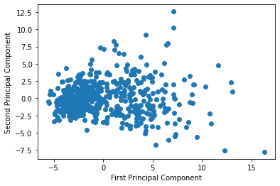
This visualization shows each data point as a function of its first and second principal components. It's not very useful in its current form.

Let's add a color scheme that modifies the color of each data point depending on whether its a malignant or benign tumor. The following code does the trick:

plt.scatter(x_pca[:,0],x_pca[:,1], c=raw_data['target'])

plt.xlabel('First Principal Component')

plt.ylabel('Second Principal Component')

This generates:

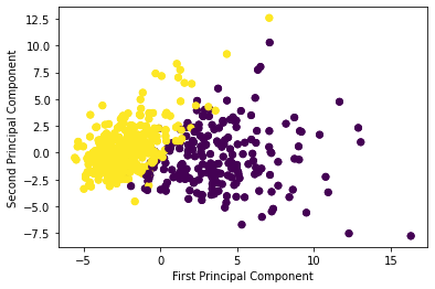
A principal component analysis with color

As you can see, using just 2 principal components allows us to accurately divide the data set based on malignant and benign tumors.

Said differently, we have maintained our ability to make accurate predictions on the data set but have dramatically increased its simplicity by reducing the number of features from 30 in the original data set to 2 principal components now.

What The Heck Is A Principal Component, Anyway?

In this tutorial (and the last one) I have often referred to "principal components", yet it's likely that you're still not sure exactly what that means. Accordingly, I wanted to spend some time providing a better explanation of what a principal component actually is.

Principal components are linear combinations of the original features within a data set. In other words, a principal component is calculated by adding and subtracting the original features of the data set.

You can use scikit-learn to generate the coefficients of these linear combination. Simply type pca.components_ and it will generate something like this:

array([[ 0.21890244,  0.10372458,  0.22753729,  0.22099499,  0.14258969,

         0.23928535,  0.25840048,  0.26085376,  0.13816696,  0.06436335,

         0.20597878,  0.01742803,  0.21132592,  0.20286964,  0.01453145,

         0.17039345,  0.15358979,  0.1834174 ,  0.04249842,  0.10256832,

         0.22799663,  0.10446933,  0.23663968,  0.22487053,  0.12795256,

         0.21009588,  0.22876753,  0.25088597,  0.12290456,  0.13178394],

       [-0.23385713, -0.05970609, -0.21518136, -0.23107671,  0.18611302,

         0.15189161,  0.06016536, -0.0347675 ,  0.19034877,  0.36657547,

        -0.10555215,  0.08997968, -0.08945723, -0.15229263,  0.20443045,

         0.2327159 ,  0.19720728,  0.13032156,  0.183848  ,  0.28009203,

        -0.21986638, -0.0454673 , -0.19987843, -0.21935186,  0.17230435,

         0.14359317,  0.09796411, -0.00825724,  0.14188335,  0.27533947]])

This is a two-dimensional NumPy array that has 2 rows and 30 columns. More specifically, there is a row for each principal component and there is a column for every feature in the original data set. The values of each item in this NumPy array correspond to the coefficient on that specific feature in the data set.

Let's investigate the first principal component as an example. It's first 2 elements are 0.21890244 and 0.10372458. This means that the equation used to calculate this component looks something like 0.21890244x1 + 0.10372458x2 + … and the other coefficients of this linear combination can be found in the pca.components_ NumPy array.

To conclude, principal component analysis is a tradeoff between simplicity and interpretability.

Using them greatly increases the simplicity of your machine learning models.

However, they also increase the difficulty of interpreting the meaning of each variable, since a principal component is a linear combination of the actual real-world variables in a data set.

How to Use Principal Component Analysis in Practice

So far in this tutorial, you have learned how to perform a principal component analysis to transform a many-featured data set into a smaller data set that contains only principal components. We've seen that this increases simplicity but decreases interpretability.

Despite all of the knowledge you've gained about principal component analysis, we have yet to make any predictions with our principal component model.

There is a reason for this. Namely, principal component analysis _must _be combined with classification models (like logistic regression or k nearest neighbors) to make meaningful predictions.

It's important to keep this in mind moving forward.

The Full Code For This Tutorial

You can view the full code for this tutorial in this GitHub repository. It is also pasted below for your reference:

import pandas as pd
import numpy as np

import matplotlib.pyplot as plt
import seaborn
%matplotlib inline

from sklearn.datasets import load_breast_cancer
raw_data = load_breast_cancer()

raw_data_frame = pd.DataFrame(raw_data['data'], columns = raw_data['feature_names'])
raw_data_frame.columns

#Standardize the data
from sklearn.preprocessing import StandardScaler
data_scaler = StandardScaler()
data_scaler.fit(raw_data_frame)
scaled_data_frame = data_scaler.transform(raw_data_frame)

#Perform the principal component analysis transformation
from sklearn.decomposition import PCA
pca = PCA(n_components = 2)
pca.fit(scaled_data_frame)

x_pca = pca.transform(scaled_data_frame)

print(x_pca.shape)
print(scaled_data_frame.shape)

#Visualize the principal components
plt.scatter(x_pca[:,0],x_pca[:,1])
plt.xlabel('First Principal Component')
plt.ylabel('Second Principal Component')

#Visualize the principal components with a color scheme
plt.scatter(x_pca[:,0],x_pca[:,1], c=raw_data['target'])
plt.xlabel('First Principal Component')
plt.ylabel('Second Principal Component')

#Investigating at the principal components
pca.components_[0]

Final Thoughts

In this tutorial, you learned how to perform principal component analysis in Python.

Here is a brief summary of the topics we discussed:

How a principal component analysis reduces the number of features in a data set
How a principal component is a linear combination of the original features of a data set
That principal component analysis must be combined with other machine learning techniques to make predictions on real data sets

Nick McCullum